Differentiable Simulation for Search

Differentiable simulation is the concept of modeling an environment's dynamics as a differentiable function. This immediately allows us to embed the environment's rollout into the computation graph of another module, allowing end-to-end differentiable training. This property has found applications in many domains. In physics, robotics, and autonomous vehicles, the dynamics often represent kinematic equations and laws of motion or energy transfer. In graphics, it is often the rendering process that is differentiable. There, differentiable rendering is at the heart of techniques like neural radiance fields and Gaussian splatting. We've previously explored how differentiable simulation can be used for control and world modeling, yet one key aspect is missing to complete the trilogy and that is test-time search. Here we'll see how differentiable simulation can be used to design efficient fast procedures that search for the best action sequence at test time.

Introduction

When a human driver notices an approaching vehicle in the rear-view mirror, they expect to see the overtaking vehicle in front of them in the next several seconds. This intuitive subconscious anticipation is a form of world modeling and enables planning - the process of selecting the right actions by predicting and assessing their likely effects. For a computational driving agent, planning is also crucial in order to drive safely and reliably across diverse scenes and conditions.

One way to perform planning is to search for the best action sequence across multiple candidates. The planning agent imagines a number of them, uses its world model to estimate their effects, rates them according to preferences and task constraints, and selects the best one. This is intuitive, yet practical questions are still plentiful. For example, should the agent consider more trajectories or focus and refine a few of them? In this context, here we'll see that differentiable simulation is well-suited for this search problem and enables very efficient planning.

Generally, developing accurate search capabilities is not easy. Intuitively, one needs three modules: a policy to suggest actions, a state predictor to predict their effect, and a critic to score them. All modules need to be accurate so the agent can both propose good actions and recognize them as being good. Previous works have attained impressive results in controlled symbolic environments where only some of these modules have to be learned [1]. In fact, the general insight is that environments where we can obtain such components nearly optimally are more suitable for successful planning. This is because a hardcoded realistic simulator used as a state predictor, or a symbolic engine used as a critic [2], is almost always more accurate than their learned counterparts, facilitating searching.

In the field of autonomous vehicles, test-time search has been underexplored, likely due to challenges like continuous action spaces, diverse realistic scenes, and limited data scale. To search efficiently, we require (i) the next-state predictor and critic to be as accurate as possible, so the agent's imagination faithfully represents a realistic probable future, and (ii) the relationship between the agent's actions and the imagined outcome to be "easy-to-model", so that a small change in the actions leads to a small change in the imagined outcome. To satisfy these we use the differentiable simulator Waymax [3] as both a next-state predictor and a critic. Its hardcoded dynamics are realistic, making any sampled Monte Carlo trajectory highly informative. By being differentiable, we can backpropagate through it and any error in the imagined outcome induces a proportional error in the agent's imagined actions. Overall, while a simulator itself provides only evaluative feedback, like in classic reinforcement learning [4], a differentiable simulator, provides instructive feedback through the loss gradients, pointing to the direction of maximal increase and allowing the agent to more efficiently search through the possible action sequences.

Here, the particular approach for test-time planning is called Differentiable Simulation for Search (DSS), shown in Fig. 1. The agent imagines a future trajectory in which it acts according to a trained policy. The trajectory is virtual and is obtained in an autoregressive manner (step by step) using the simulator. Subsequently, the simulator rates the trajectory, based on for example whether there are any collisions or offroad events, and a planning loss is computed. The gradients of this loss propagate through the differentiable dynamics in a manner similar to backpropagation-through-time (BPTT) and reach the ego-vehicle's actions, updating them towards an optimum. The optimized actions can then be executed in the real world, thereby forming a real physical trajectory.

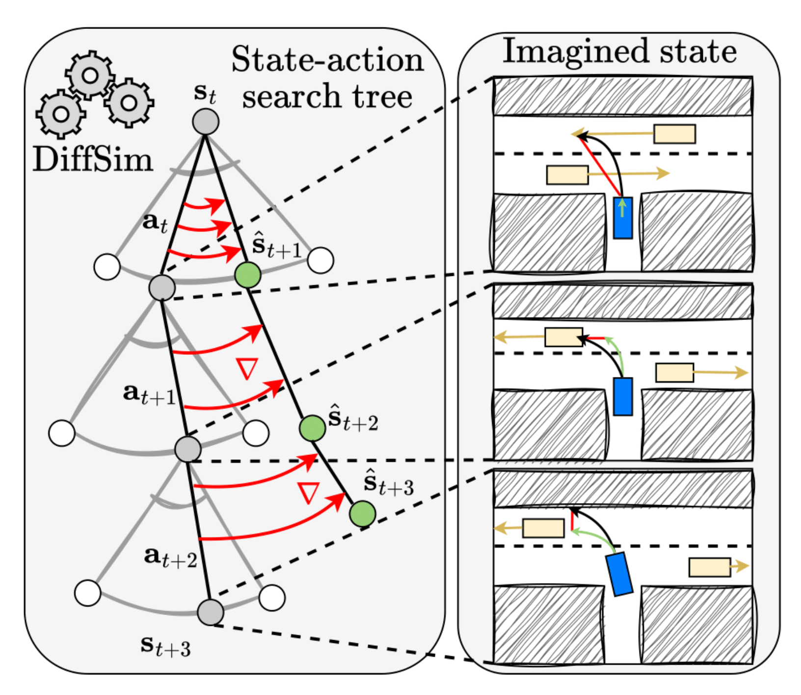
DSS — Figure 1: Differentiable simulation for search. The left panel shows the state-action tree in which the agent searchers for the best action sequence. The right panel shows individual states from it. To select the current action, the agent uses a differentiable simulator to imagine a future trajectory ($\mathbf{s}_t, ..., \mathbf{s}_{t+3}$, gray circles), sampled from a distribution of possible states (arcs, white circles). The imagined trajectory is refined (red) using gradient descent towards an optimal one ($\hat{\mathbf{s}}_{t+1}, ..., \hat{\mathbf{s}}_{t+3}$, green circles).

The DSS approach is designed for single-agent control. A conceptual requirement is that within the virtual future other agents should evolve according to how the ego-vehicle imagines them. From its perspective, this is natural, given that everything is controllable within one’s own imagination.

From the perspective of the Waymax, however, in order to enable single-agent planning for the ego-vehicle, one needs to perform multiagent control virtually to predict other agent’s actions and evolve them to their future locations. Waymax works by replaying the historical real-world scenarios from the Waymo Open Motion Dataset (WOMD) [5]. Those agents not controlled by a learned, user-provided policy are evolved according to their historic motion, which the ego-vehicle is not supposed to see. Thus, to avoid a potential data leakage, in Waymax the same policy that controls the ego-vehicle should also control the other vehicles, only within the imagined future. In that sense, the multi-agent control is like the ego-vehicle imagining the future motion of the other agents.

To run such a planner in a real vehicle, one would need a sensing stack with (i) state estimation software that initializes the simulator state from real sensory data (surrounding cameras, LiDAR, IMUs), keeps track of appearing and disappearing objects, receives navigation, and (ii) state simulation software, which steps the dynamics forward and generates the virtual trajectories. While Waymax only provides state simulation, adopting the WOMD scenarios and their 9 second episodes allows us to sidestep the need to build state estimation ourselves, facilitating the study of the planning task in isolation.

Training - Analytic Policy Gradients

Notation. We represent the set of all states as $\mathcal{S}$ and that of the actions as $\mathcal{A}$. The simulator is abstracted as a pure, stateless differentiable function, $\text{Sim}: \mathcal{S} \times \mathcal{A} \rightarrow \mathcal{S}$, that maps state-action pairs to next states, $\text{Sim}(\mathbf{s}_t, \mathbf{a}_t) \mapsto \mathbf{s}_{t + 1}$. A trajectory is a sequence of state-action pairs $(\mathbf{s}_0, \mathbf{a}_0, \mathbf{s}_1, \mathbf{a}_1, ..., \mathbf{s}_T)$. We can extract agent locations $(\mathbf{x}_0, \mathbf{x}_1, ..., \mathbf{x}_T)$ and action sequences $(\mathbf{a}_0, ..., \mathbf{a}_{T-1})$ from it. We denote an action of the $e$go-vehicle as $\mathbf{a}_t^e$, and an action of all $o$ther agents (of which there are up to 128 in any episode) as $\mathbf{a}_t^{o}$. Actions are vector-valued with a dimension $A$ and represent acceleration and steering in our setting.

The DSS agent requires a learned stochastic policy $\pi_\theta$ to model agent behavior. We use Analytic Policy Gradients (APG) to learn a realistic action distribution from historical expert driver trajectories. Specifically, we can train on the WOMD scenarios within Waymax. In each scenario the agent performs a rollout, after which the full obtained trajectory $(\mathbf{s}_0, ..., \mathbf{s}_T)$ is supervised with the expert human driver one, $(\hat{\mathbf{s}}_0, ..., \hat{\mathbf{s}}_T)$. Gradients flow through the dynamics, similar to BPTT:

$$ \begin{equation} \begin{aligned} \min_\theta \ \mathcal{L}_\text{train} &= {\lVert\mathbf{s}_t - \hat{\mathbf{s}}_t\rVert}_2^2 \\ \text{ with } \mathbf{s}_t &= \text{Sim}(\mathbf{s}_{t-1}, \pi_\theta(\mathbf{s}_{t-1})). \end{aligned} \end{equation} $$

Action selection. The policy $\pi_\theta$ is stochastic and is parametrized as a Gaussian mixture with six components. To encourage action multimodality during training, actions for the rollout are selected by sampling not from the entire Gaussian mixture, but only from that one component that will bring the ego-vehicle closest to the next expert state [6]. We use the simulator to find that component efficiently. The error signals during backpropagation reach only this component, instead of all of them. This allows the policy to sample diverse actions, which is beneficial for searching at test time.

Recurrent architecture. Since the policy is recurrent, its hidden state encapsulates the entire history of observations, represented as $\pi_\theta(\mathbf{a}_t | \mathbf{s}_{\le t})$. For computational efficiency during training we only control the ego-vehicle, while the other agents' states evolve according to their historic motion. However, at test time the policy could be used to control also the other agents. By extracting state observations from the perspective of all agents we can compute all actions in parallel. We overwrite the notation as $\mathbf{a}_t^e, \mathbf{a}_t^o = \pi_\theta(\mathbf{x}_{\le t}^e, \mathbf{x}_{\le t}^o)$, where $\mathbf{x}_t^e$ and $\mathbf{x}_t^o$ indicate the $e$go and $o$ther agents' positions at time $t$. With this architecture we have a policy that can be effectively simulate the behavior of all agents. One particular limitation here is that the same statistical patterns learned for vehicle motion will be used for controlling all all agents, even those with seemingly different motion patterns (e.g. pedestrians). This is more of a conceptual than an experimental problem.

Testing - Differentiable Simulation for Search

The planning algorithm at test time, called Differentiable Simulation for Search (DSS), is shown in Fig. 2. To select the current action, the ego-agent imagines $K$ future trajectories, each of length $T$ steps. They are generated autoregressively by using the trained policy $\pi_\theta$ to compute actions for both the ego- and the other agents, while the simulator is used to compute their next states, in lines 3-5. Having obtained the $K$ trajectories, we compute a loss function over the ego positions, line 6. With DiffSim, in lines 7 and 9 we can compute the gradients of the loss with respect to the first ego-action and perform a single gradient descent step to improve it. Since the algorithm is based on sampled imaginary rollouts, the final selected action is a weighted average of the optimized first actions from these rollouts, where actions in trajectories with lower losses have higher weights.

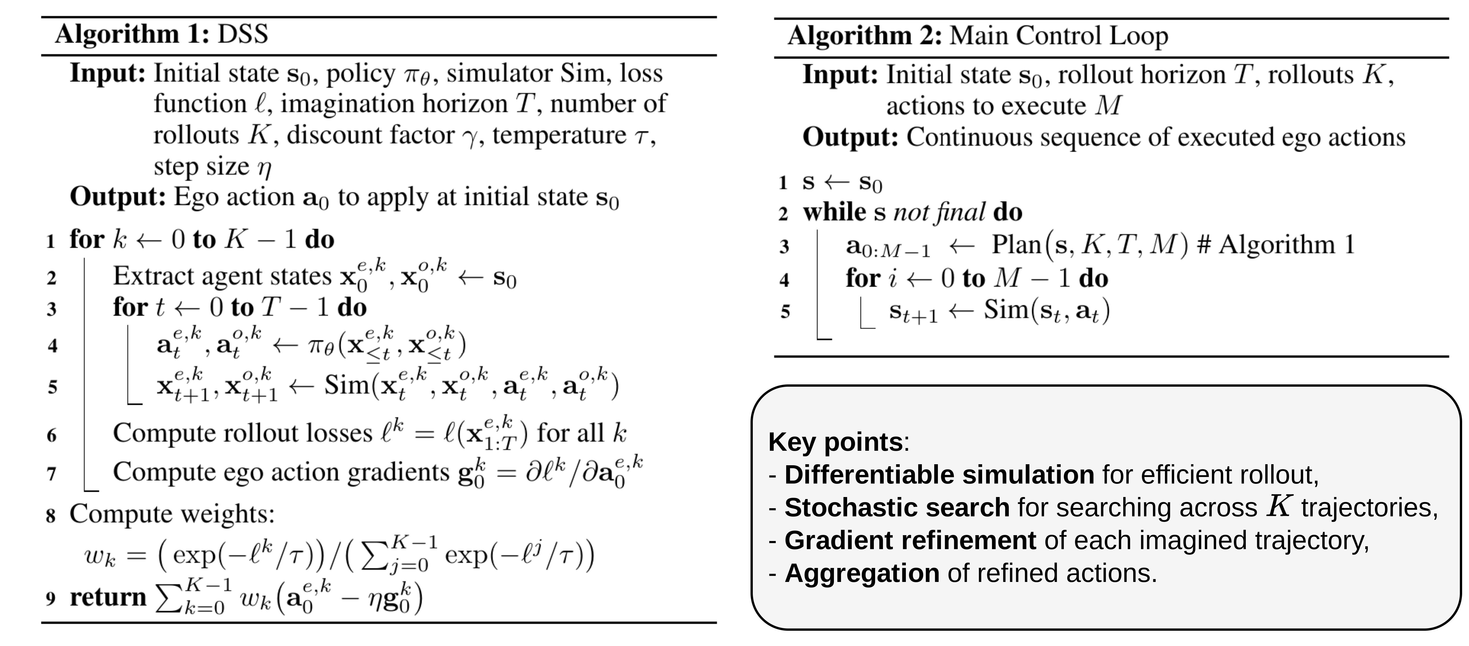
Figure 2: DSS pseudocode. Algorithm 1 details how the agent refines its action by searching within the virtual, imagined future. Algorithm 2 presents the main control loop that generates the physical trajectory.

Flexibility. Alg. 1 encompasses a full set of possible behaviors for how the agent can plan its action at test time. The setting $K=1, T=1, \eta = 0$ represents a reactive agent that drives by relying on the trained policy $\pi_\theta$. If $K=1$ but $\eta > 0$, the agent uses the differentiability of the simulator to optimize its actions, as the gradient step size $\eta$ is positive, but does not use the simulator to perform Monte Carlo search. We call this setting reactive with gradients. If $K > 1$ and $\eta = 0$ the agent uses multiple Monte Carlo rollouts to search for the right actions but does not use gradient descent to optimize them. This setting is called simulator as a critic, because the simulator computes trajectories and losses, but its differentiability is not used. Finally, the full setting differentiable simulator as a critic is enabled when gradients are used to optimize the actions, i.e. $\eta > 0$, and multiple rollouts are used to search, i.e. $K > 1$.

Control loop. The imagined trajectories in Alg.1 are virtual - they represent the future as predicted by the ego-agent's policy. Algorithm 2 provides the main loop for obtaining a real, physical trajectory, over which the evaluation metrics are calculated. Specifically, instead of planning out only the first action, we optimize and execute the first $M$ imagined actions, after which the ego-vehicle has to re-plan. In line 5, only the ego-agent is controlled by the policy's optimized actions. This is in contrast to line 5 in Alg. 1 where all agents are controlled. The overall effect is that Alg. 1 shows how the ego-vehicle optimizes its own actions within the virtual, imagined dynamics, which inherently involves multi-agent control in order to imagine the other agents' motions, while Alg. 2 is used to obtain the real physical trajectories, where only the ego-vehicle is controlled by the policy $\pi_\theta$.

Computational cost. When re-planning once every $M$ steps, the reaction time to any observation can be up to $M$ steps. Re-planning once every $3$ steps corresponds to a reaction time of at most $0.3$ seconds (at 10 frames per second). The total computational cost, in number of policy calls, is $O(LKTN/M)$ where $L$ is the length of the physical trajectory, and $N$ is the maximum number of actors in the scene. For Waymax, where $L=90$ and $N=128$, and when $M=3$, $K=1$, and $T=20$, this runs at $1.67$ seconds per scenario on a single RTX3090 GPU. Thus, a full scenario long $90$ timesteps, or $9$ seconds of historical real driving, is processed in $1.67$ seconds - effectively real-time. I'm honestly amazed that this kind of plannig is feasible to run in a real car.

Results

Now, without going over all the little experiments and evaluation details, the main results are that:

Planning in general helps compared to reactively following the trained policy at test time.
Stochastic search helps - a higher number of imagined trajectories $K$ in most cases improves performance because the agent gets to see more possible future situations and can experience, by chance, better actions.
Gradient refinement helps - even a single step of gradient descent per real timestep can improve performance. The main parameter controlling the effect here is the step size $\eta$. If it's too low, refinement has little to no impact. If it's moderate, it helps. If it's too large, it causes gradient overshooting, hurting performance.
A longer planning horizon $T$ generally improves performance, depending on the planning loss.
The planning loss $\ell$ in line 6 is crucial. It models the planning problem and could represent different settings like tracking or autonomous path planning.
Replanning often (lower $M$) improves performance but directly increases compute time.

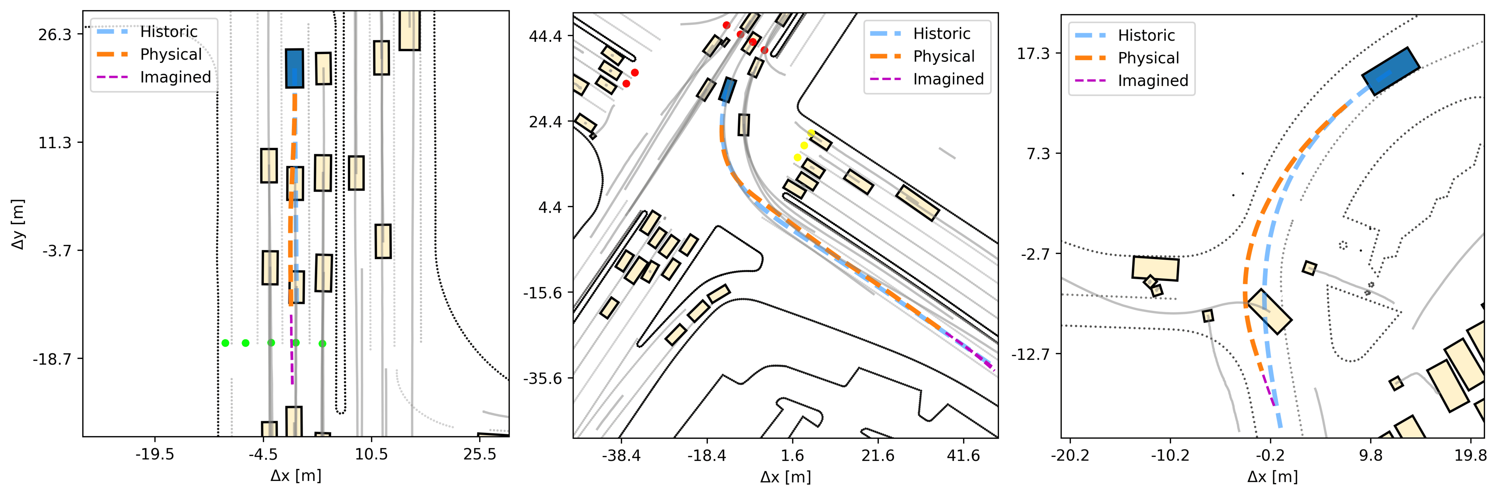
Figure 3: Qualitative samples from the DSS agent. The ego-vehicle is blue. All boxes are shown at their initial positions and the gray lines indicate their future motion (crossing lines do not imply collisions). Red dots are red lights. The ego-agent accurately navigates the intersections and turns by periodically planning out its actions through imagination of the future (shown in purple).

Fig. 3 shows qualitative test-time samples of how the ego-agent drives. We plot the imagined future as a purple dashed line at a single point of time towards the end of the trajectories. Generally, behavior is accurate, precise and humanlike. The agent can accurately follow its lane, turn at intersections, accelerate and decelerate according to the context. The route conditioning is important to determine its intended final destination. Here the agent sees the last $(x, y)$ waypoint from the historic trajectory and uses it to direct its steering and acceleration. If we only use, say, the heading angle toward the final point, then we'd expect more longitudinal errors.

In general, there is an important distinction between encouraging the agent to reach a destination at a particular time, vs at any time. If the planning loss is the $L_2$ distance between the last imagined $(x, y)$ location 1 second in the future and the last historic $(x, y)$ waypoint, say, 5 seconds in the future, this is problematic. It creates a temporal misalignment that will cause the agent to over-accelerate. In those cases, it's better to encourage any safe progress towards the target, even if it is delayed to some extent. Yet, this is where things get tricky, as it should not be delayed too much... This type of nuanced design of the planning objective is far from solved. That being said, we don't need to solve it to see the merits of the DSS planning method. The bottom line is that differentiable simulation can be helpful also when doing test-time search.

References

[1] Silver, David, et al. Mastering the game of Go with deep neural networks and tree search. nature 529.7587 (2016): 484-489.
[2] Trinh, Trieu H., et al. Solving olympiad geometry without human demonstrations. nature 625.7995 (2024): 476-482.
[3] Gulino, Cole, et al. Waymax: An accelerated, data-driven simulator for large-scale autonomous driving research. Advances in Neural Information Processing Systems 36 (2023): 7730-7742.
[4] Sutton, Richard S., and Andrew G. Barto. Reinforcement learning: An introduction. Vol. 1. No. 1. Cambridge: MIT press, 1998.
[5] Ettinger, Scott, et al. Large scale interactive motion forecasting for autonomous driving: The waymo open motion dataset. Proceedings of the IEEE/CVF international conference on computer vision. 2021.
[6] Nayakanti, Nigamaa, et al. Wayformer: Motion forecasting via simple & efficient attention networks. arXiv preprint arXiv:2207.05844 (2022).