Analytic Policy Gradients
Current methods to learn controllers for autonomous vehicles (AVs) focus on behavioral cloning, where agents learn to mimic the actions obtained from an expert trajectory. Being trained only on exact historic data, the resulting agents often generalize poorly when deployed to novel scenarios. Simulators provide the opportunity to go beyond offline datasets, but they are still treated as complicated black boxes, only used to update the global simulation state. As a result, these RL algorithms are slow, sample-inefficient, and prior-agnostic. Instead, if these simulators are differentiable, they can be included into an end-to-end training loop, turning their hard-coded world dynamics into useful inductive biases for the model. Here we explore the differentiable Waymax simulator and use analytic policy gradients to train AV controllers on the large-scale Waymo Open Motion Dataset (WOMD). This allows us to learn robust, accurate, and fast policies only using gradient descent.
Introduction
In policy gradients one optimizes the policy function directly by maximizing the likelihood of actions corresponding to high rewards. This works by purposefully trying out different actions, collecting their rewards, and then increasing the likelihood of the actions according to their rewards. The optimization process is stochastic, difficult and often over-reliant on the rewards, which for realistic settings like driving, may be prohibitively hard to define. Another alternative are model-based methods, which learn the dynamics of the environment, allowing them to plan at test-time. Their training is stable, but slow to execute. Additionally, the precision of the policy is bounded by the precision of the learned dynamics. Finally, imitation learning attempts to learn directly from expert actions. It simply supervises the policy's predicted actions with the expert ones, which often may be costly to obtain in large quantities or lack sufficient diversity.
In settings where the environment dynamics are known one would likely be able to harvest the best aspects from each of these methods. In fact, if the dynamics are differentiable, then effectively the entire rollout becomes differentiable and one can optimize the policy directly using gradient descent, just via supervision from expert agent trajectories. The benefits of this are: 1) Obtaining an explicit policy for continuous control, 2) Fast inference, since there is no planning at test time. 3) Unbounded policy precision, due to the dynamics not being approximated, 4) Facilitating more grounded learning by incorporating the dynamics directly into the training loop.
Waymax was recently introduced as a differentiable, large-scale autonomous driving simulator [1]. It allows us to replay the episodes from the Waymo Open Motion Dataset (WOMD) [2], a large-scale driving dataset collected by expert human drivers, and composed of thousands of driving trajectories from diverse cities and situations. Each episode designates a particular vehicle as the ego-agent and contains static data, e.g. roadgraph with lanes, crossings, intersections, markings, and dynamic data, e.g. the historical trajectories of the ego- and all other vehicles. When replaying these episodes, Waymax enables us to manually control the agents, in which case their simulated trajectories could deviate from the historical (ground-truth) ones.
In this post, we'll explore how Waymax's differentiability can be used to train controllers using Analytic Policy Gradients (APG), reaping all the benefits mentioned above. We'll see that the resulting policies are precise and accurate, often very human-like.
Method
In essence, a differentiable environment allows us to backpropagate gradients through it and directly optimize the policy. The resulting method broadly falls into the analytic policy gradients (APG) type of algorithms. In our setting we assume we are provided with widely-available expert trajectories \( \{ \hat{\mathbf{s}}_t \}_{t=1}^T\), instead of rewards, or expert actions \(\{\hat{\mathbf{a}}\}_{t=1}^T\). The goal is to train the policy \(\pi_\theta\) so that upon a roll-out, it reproduces the expert trajectory:
Here, and in what follows, \(\hat{\textbf{s}}_t\) and \(\hat{\textbf{a}}_t\) refer to ground truth states and actions while \(\textbf{s}_t\) and \(\textbf{a}_t\) are the corresponding simulated states and actions. The sequence of states \( \{ \mathbf{s}_t \}_{t=1}^T\) forms a trajectory.
This optimization task is difficult because trajectories are generated in a sequential manner with current states depending on previous actions, which themselves recursively depend on previous states. Additionally, \(\nabla_\theta \mathcal{L}\) (shown here for only one of its additive terms) has the form
which multiplicatively composes multiple derivatives \({\partial \mathbf{s}_{t+1}}/{\partial \mathbf{a}_{t}}\), corresponding to the environment dynamics, and mixes them together with the policy derivatives \({\partial \mathbf{a}_t} / {\partial \mathbf{s}_{t}}\). This is the core of differentiable simulation, it embeds the newly-available dynamics gradients within a broader training loop, in this case that of the policy \(\pi_\theta\).
Application setting. Ultimately, for motion perception and planning in autonomous vehicles, we are interested in multi-modal trajectory prediction. Given a short history segment for all agents in the scene, we want to obtain \(K\) modes, or probable trajectories, for the future of each agent. Given a simulator, we can learn a stochastic policy, or controller, for the agents. Then, we can perform \(K\) roll-outs, obtaining \(K\) future trajectories. Hence, in the presence of a simulator, the task of trajectory prediction reduces to learning a policy \(\pi_\theta: \textbf{s}_t \mapsto \textbf{a}_t\) to control the agents.
Obtaining gradients. We apply our APG method in the Waymax simulator [1]. Being implemented in Jax [3], it is relatively flexible in choosing which variable to differentiate and with respect to what. All objects of interest are tensors and the bicycle dynamics (themselves realistic and nonlinear) are differentiable. That being said, many of the obtainable derivatives are not meaningful. For example,
- The derivatives of future agent locations with respect to the current traffic light state are all zero, because the agent locations and, in general, the simulator dynamics do not depend on the roadgraph or the traffic lights.
- Certain metrics such as collision or offroad detection are boolean in nature. Other objects such as traffic lights have discrete states. These are problematic for differentiation.
What is meaningful and useful is to take the gradients of future agent locations with respect to current actions. These are precisely the derivatives needed for the optimization above and hence we focus on them. To obtain them, one needs to ensure that the relevant structures in the code are registered in Jax's pytree registry, so that any tracing, just-in-time compilation, or functional transformations like grad can work on them.
Moreover, it's generally useful to adapt the bicycle dynamics to be gradient-friendly. This includes adding a small epsilon to the argument of a square root to avoid the case when its input is 0, as well as adapting the yaw angle wrapping, present in many similar settings, to use arctan2 instead of mod, which makes the corresponding derivatives continuous.

Dense trajectory supervision. Obtaining the gradients of the environment dynamics opens up technical questions of how to train in such a setup. One can supervise the rolled-out trajectory only at the final state and let the gradients flow all the way back to the initial state. Since this does not supervise the path taken to the objective, in our experiments we densely supervise all states in the collected trajectory with all states in the GT trajectory.
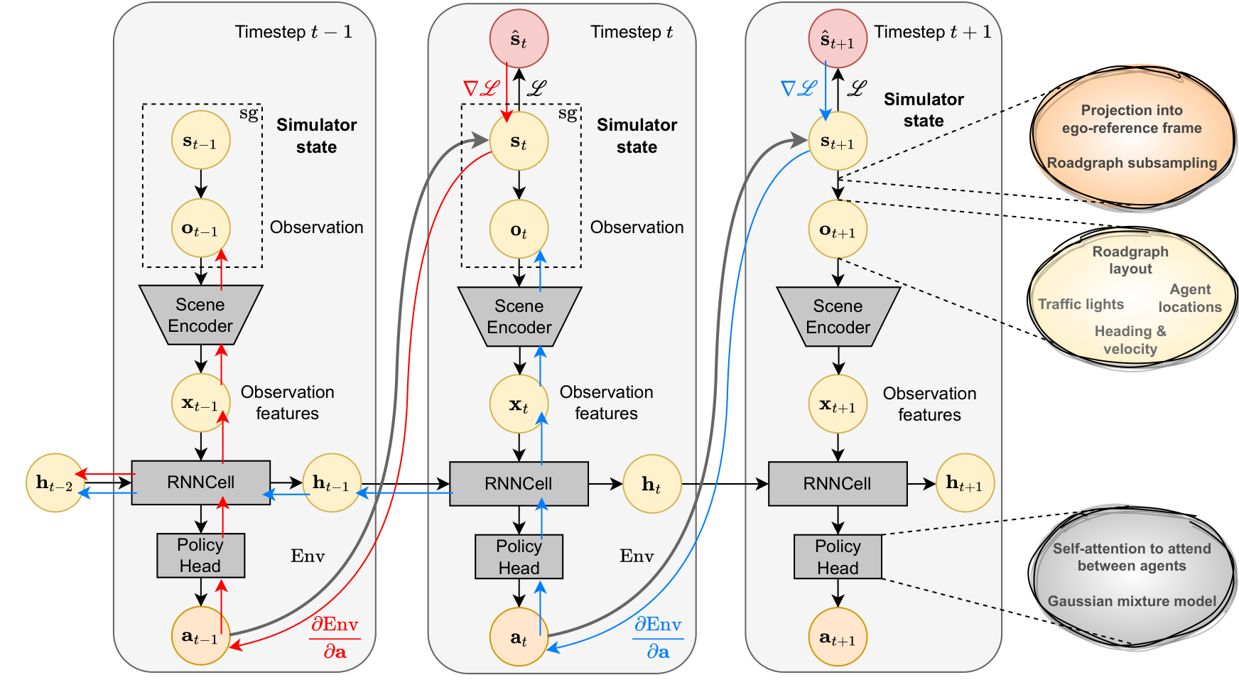
Gradient detaching. Dense supervision allows us to detach the gradients at the right places, as shown in the third part of Fig. 1. Here, when we obtain \(\mathbf{s}_t\), we calculate the loss and backpropagate through the environment dynamics obtaining \(\partial \mathbf{s}_t / \partial \mathbf{a}_{t - 1}\) without continuing on to previous steps. This makes training slower, since gradients for the earlier steps do not accumulate, as in a RNN, but effectively cuts the whole trajectory into many \((\textbf{s}_t, \textbf{a}_t, \textbf{s}_{t+1})\) transitions which can be treated independently by the optimization step. This allows off-policy training - a key aspect of the setup.

Model overview. The agent architecture is presented in Figure 2. For training, we roll-out a full trajectory and supervise with the GT one. The gradients flow back through the differentiable dynamics, policy and scene encoder, and continue back to the previous scene contexts using an RNN hidden state. We detach the previous simulator state for both necessity and flexibility so that the state transitions on which we compute the loss can be different from the transitions executed during roll-out. Nonetheless, because of the RNN setup, current step dynamics gradients can backpropagate and mix with earlier policy gradients.
Optimization difficulty. Differentiating through a stochastic policy requires that the actions be reparametrized. But every reparametrization leads to stochastic gradients for those layers before it. And when we compose multiple sampling operations sequentially, such as in the computation graph of the entire collected trajectory, the noise starts to compound and may overwhelm the actual signal from the trajectory steps, making the optimization more noisy and difficult. To address this, one could implement incremental training where we periodically "reset" the simulated state back to the corresponding log state. This ensures that data-collection stays around the GT trajectory, instead of far from it. The frequency of resetting decays as training progresses.
Agent processing. For multi-agent simulation it is useful to slightly adapt our architecture to allow training with \(N\) agents but evaluating with \(M\). It's common to adopt a small transformer that forces each agent to attend to the other ones in parallel. However, at the last transformer block we can use a fixed number of learned queries which attend over the variable number of agent keys and values, effectively soft-clustering them, and becoming independent of their number. This allows us to train with 32 agents but evaluate with 128, as required for example by the Waymo Sim Agents challenge [4].

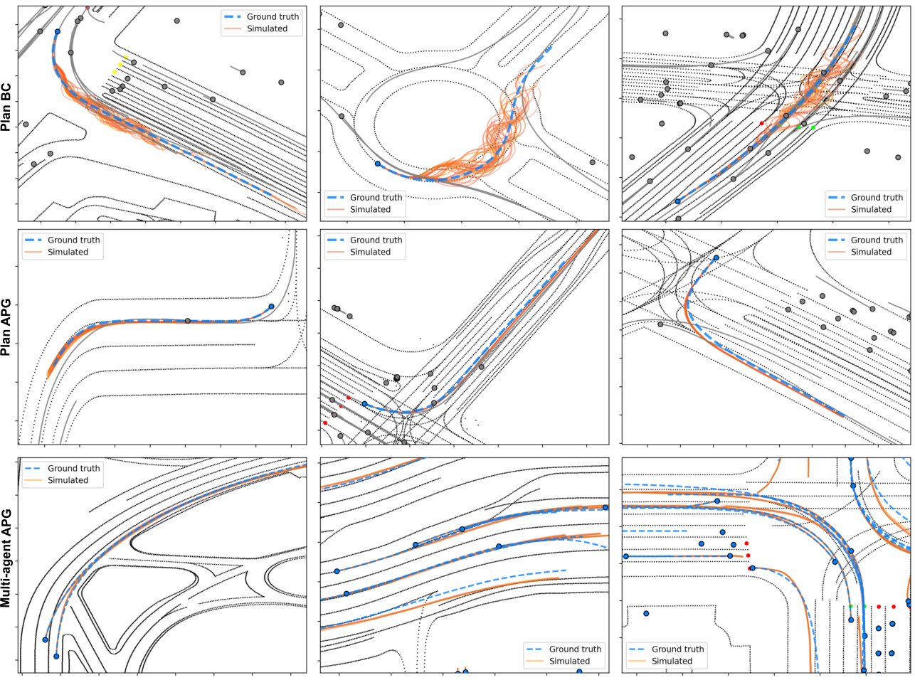
Qualitative study. We showcase sample trajectories from the APG method in Fig. 3 and observe that in the planning setting (single-agent control) APG realizes accurate stochastic trajectories. Errors are mostly longitudinal and occur from not predicting the correct acceleration, not the steering. This is often explained by the type of route conditioning that marks the intended driving direction. If the agent is only provided directions (steer left, right), naturally it won't know when to accelerate or decelerate. Steering errors are more prevalent in the behavior cloning (BC) models and causes the agent there to swerve. In multi-agent (MA) settings, where the same policy controls all agents, the MA-APG trajectories are relatively less accurate because, unlike in planning, when all agents are controlled, any prediction will have an effect on any agent, making training more difficult. Nonetheless, performance is quite good, showing that the benefit of a differentiable simulator, which is the ability to train policies in a supervised manner, is indeed useful, leading to more accurate, robust and potentially safer executed trajectories.
References
[1] Gulino, Cole, et al. Waymax: An accelerated, data-driven simulator for large-scale autonomous driving research. Advances in Neural Information Processing Systems 36 (2024).
[2] Ettinger, Scott, et al. Large scale interactive motion forecasting for autonomous driving: The waymo open motion dataset. Proceedings of the IEEE/CVF International Conference on Computer Vision. 2021.
[3] Bradbury, James, et al. JAX: Composable Transformations of Python+NumPy Programs. Version 0.3.13, 2018.
[4] Montali, Nico, et al. The waymo open sim agents challenge. Advances in Neural Information Processing Systems 36 (2024).