Analytic World Models

Differentiable simulators have recently shown great promise for training autonomous vehicle controllers. Being able to backpropagate through them, they can be placed into an end-to-end training loop where their known dynamics turn into useful priors for the policy to learn, removing the typical black box assumption of the environment. So far, these systems have only been used to train policies. However, this is not the end of the story in terms of what they can offer. They can also be used to train world models. Specifically, in this post we propose and explore three new task setups that allow us to learn next state predictors, optimal planners, and optimal inverse states. Unlike analytic policy gradients (APG), which requires the gradient of the next simulator state with respect to the current actions, the proposed setups rely on the gradient of the next state with respect to the current state. We call this approach Analytic World Models (AWMs).

Introduction

Differentiable simulation has emerged as a powerful tool to train controllers and predictors across different domains like physics, graphics, and robotics. Within the field of autonomous vehicles (AVs), we've already looked at how differentiable motion dynamics can serve as a useful stepping stone for training robust and realistic vehicle policies. The framework is straightforward and bears similarity to backpropagation through time - it involves rolling out a trajectory and supervising it with a ground-truth (GT) expert one. The process is sample-efficient because the gradients of the dynamics automatically guide the policy toward optimality and there is no search involved, unlike when the environment is treated as black box.

Yet, this has only been explored for single policies, which are reactive [1] in their nature - at test-time they simply associate an action with each observation without providing any guarantee for their expected performance. Unlike them, model-based methods use planning at test time, which guarantees to maximize the estimated reward. They are considered more interpretable compared to model-free methods, due to the simulated world dynamics, and more amenable to conditioning, which makes them potentially safer. They are also sample-efficient due to the self-supervised training. Consequently, the ability to plan at test time is a compelling requirement towards accurate and safe autonomous driving.

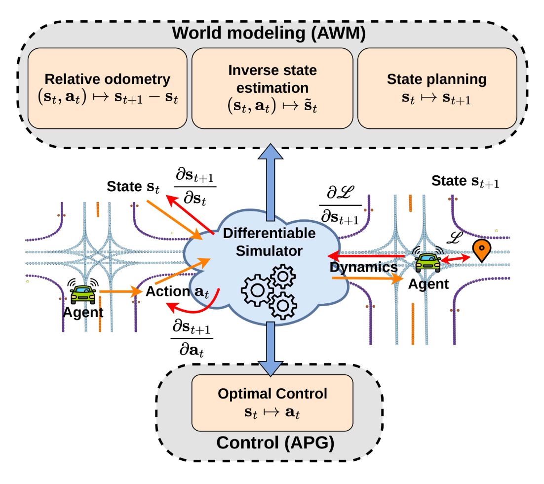
An open question is whether model-based methods can be trained and utilized in a differentiable environment, and what would be the benefits of doing so. Let's explore this question here. Naturally, planning requires learning a world model, but the concept of a world model is rather nuanced, as there are different ways to understand the effect of one's own actions. Fig. 1 shows our approach, which uses the differentiability of the simulator to formulate three novel tasks related to world modeling. First, the effect of an agent's action could be understood as the difference between the agent's next state and its current state. If a vehicle's state consists of its position, yaw, and velocity, then this setup has an odometric interpretation. Second, an agent could predict not an action, but a desired next state to visit, which is a form of state planning. Third, we can ask "Given an action in a particular state, what should the state be so that this action is optimal?", which is another form of world modeling but also an inverse problem.

Thus, we are motivated to understand the kinds of tasks solvable in a differentiable simulator for vehicle motion. Policy learning with differentiable simulation is called Analytic Policy Gradients (APG). Similarly, we call the proposed approach Analytic World Models (AWMs). It is intuitive, yet distinct from APG because APG requires the gradients of the next state with respect to the current actions, while AWM requires the gradients of the next state with respect to the current state.

The benefit of using a differentiable environment for solving these tasks is twofold. First, by not assuming black box dynamics, one can avoid searching for the solution, which improves sample efficiency. Second, when the simulator is put into an end-to-end training loop, the differentiable dynamics serve to better condition the predictions, leading to more physically-consistent representations, as evidenced from other works. This happens because the gradients of the dynamics get mixed together with the gradients of the predictors. More generally, similar to how differentiable rendering allows us to solve inverse graphics tasks, differentiable simulation allows us to solve new inverse dynamics tasks.

Having established the world modeling tasks, we can use them for planning at test time. Specifically, we formulate a method based on model-predictive control (MPC), which allows the agent to autoregressively imagine future trajectories and apply the proposed world modeling predictors on their imagined states. Thus, the agent can efficiently compose these predictors in time. Note that this requires another world modeling predictor - one that predicts the next state latent sensory features from the current ones. This is the de facto standard world model [2]. Its necessity results only from the architectural design, to drive the autoregressive generation. Contrary to it, the predictions from our three proposed tasks are interpretable and meaningful, and represent a step towards the goal of having robust accurate planning for driving.

We'll use Waymax [3] as our simulator of choice, due to it being fully differentiable and data-driven. The scenarios are instantiated from the large-scale Waymo Open Motion Dataset (WOMD) [4] and are realistic in terms of roadgraph layouts and traffic actors.

Method

Now, let's look at the different task formulations for learning in a differentiable simulator. We'll then cover the architecture and planning aspects.

Notation. In all that follows we represent the current simulator state with $\mathbf{s}_t$, the current action with $\mathbf{a}_t$, the log (expert) state with $\hat{\mathbf{s}}_t$, the log action with $\hat{\mathbf{a}}_t$. The simulator is a function $\text{Sim}: \mathcal{S} \times \mathcal{A} \rightarrow \mathcal{S}$, with $\text{Sim}(\mathbf{s}_t, \mathbf{a}_t) \mapsto \mathbf{s}_{t + 1}$, where the set of all states is $\mathcal{S}$ and that of the actions $\mathcal{A}$.

APG. We know that a differentiable simulator can turn the search problem of optimal policy learning into a supervised one. Here the policy $\pi_\theta$ produces an action $\mathbf{a}_t$ from the current state, which is executed in the environment to obtain the next state $\mathbf{s}_{t+1}$. Comparing it to the log-trajectory $\hat{\mathbf{s}}_{t+1}$ produces a loss, whose gradient is backpropagated through the simulator and back to the policy:

The key gradient here is that of the next state with respect to the current agent actions $\frac{\partial \mathbf{s}_{t+1}}{\mathbf{a}_t}$. The loss is minimized whenever the policy outputs an action equal to the inverse kinematics $\text{InvKin}(\mathbf{s}_t , \hat{\mathbf{s}}_{t+1})$. To obtain similar supervision without access to a differentiable simulator, one would need to supervise the policy with the inverse kinematic actions, which are unavailable if the environment is considered a black box. Hence, this is an example of an inverse dynamics problem that is not efficiently solvable without access to a known environment, in this case to provide inverse kinematics.

Relative odometry. In this simple setting a world model $f_\theta : \mathcal{S} \times \mathcal{A} \rightarrow \mathcal{S}$ predicts the next state $\mathbf{s}_{t+1}$ from the current state-action pair $(\mathbf{s}_t, \mathbf{a}_t)$. Here, a differentiable simulator is not needed to learn a good predictor. One can obtain $(\mathbf{s}_t, \mathbf{a}_t, \mathbf{s}_{t+1})$ tuples simply by rolling out a random policy and then supervising the predictions with the next state $\mathbf{s}_{t+1}$. Nonetheless, we provide a formulation for bringing the simulator into the training loop of this task:

Here, the world model $f_\theta$ takes $(\mathbf{s}_{t}, \mathbf{a}_t)$ and returns a next-state estimate $\tilde{\mathbf{s}}_{t+1}$. We then feed it into an inverse simulator $\text{Sim}^{-1}$ which is a function with the property that $\text{Sim}^{-1}( \text{Sim}(\mathbf{s}_t, \mathbf{a}_t), \mathbf{a}_t) = \mathbf{s}_t$. This output is compared with the current $\mathbf{s}_t$. The loss is minimized when $f_\theta$ predicts exactly $\mathbf{s}_{t+1}$, thus becoming a predictor of the next state.

I implemented the inverse simulator for the bicycle dynamics in Waymax [3], however observed that it is problematic in the following sense. The velocities $v_x$ and $v_y$ are tied to the yaw angle of the agent through the relationship $v_x = v \cos \phi$ and $v_y = v \sin \phi$, where $\phi$ is the yaw angle and $v$ is the current speed. However, at the first simulation step, due to the WOM dataset [4] being collected with noisy estimates of the agent state parameters, the relationships between $v_x$, $v_y$, and $\phi$ do not hold. Thus, the inverse simulator produces incorrect results for the first timestep.

For this reason, one can provide another formulation for the problem that only requires access to a forward simulator and thus avoids the problem of inconsistent first-steps:

Here, $f_\theta$ predicts the relative state difference that executing $\mathbf{a}_t$ will bring to the agent. One can verify that the loss is minimized if and only if the prediction is equal to $\mathbf{s}_{t+1} - \mathbf{s}_t$. This can still be interpreted as a world model where $f_\theta$ learns to estimate how an action would change its relative state. Since the time-varying elements of the agent state consist of $(x, y, v_x, v_y, \phi)$, this world model has a clear relative odometric interpretation. Learning such a predictor without a differentiable simulator will prevent the gradients of the environment dynamics from mixing with those of the network.

Inverse dynamics and inverse kinematics. Given a tuple $(\mathbf{s}_t, \mathbf{a}_t, \mathbf{s}_{t + 1})$, one can learn inverse dynamics $(\mathbf{s}_{t+1}, \mathbf{a}_t) \mapsto \mathbf{s}_t$ and inverse kinematics $(\mathbf{s}_{t}, \mathbf{s}_{t+1}) \mapsto \mathbf{a}_t$ without a differentiable simulator, which is useful for exploration \cite{pathak2017curiosity}. Formulations that involve the simulator are also possible. We'll skip their formulations, as it's very similar to the ones already presented.

Optimal planners. We call the network $f_\theta: \mathcal{S} \rightarrow \mathcal{S}$ with $\mathbf{s}_t \mapsto \mathbf{s}_{t+1}$ a planner because it plans out the next state to visit from the current one. Unlike a policy, which selects an action without explicitly knowing the next state, the planner does not execute any actions. Hence, until an action is executed, its output is inconsequential. We consider the problem of learning an optimal planner. With a differentiable simulator, as long as we have access to the inverse kinematics, we can formulate the optimisation as:

Here, $f_\theta$ predicts the next state to visit as an offset to the current one. The action that reaches it is obtained using the inverse kinematics. After executing the action we directly supervise with the optimal next state. The gradient of the loss goes through the simulator, the inverse kinematics, and finally through the state planner network. Note that with a black box environment we can still supervise the planner directly with $\hat{\mathbf{s}}_{t+1}$, but a black box does not provide any inverse kinematics, hence there is no way to perform trajectory rollouts, unless with a separate behavioral policy.

Inverse optimal state estimation. We now consider the following task \emph{"Given $(\mathbf{s}_t, \mathbf{a}_t)$, find an alternative state for the current timestep $t$ where taking action $\mathbf{a}_t$ will lead to an optimal next state $\hat{\mathbf{s}}_{t+1}$"}. We formulate the problem as

Here $f_\theta$ needs to estimate the effect of the action $\mathbf{a}_t$ and predict a new state $\tilde{\mathbf{s}}_t$, relatively to the current state $\mathbf{s}_t$, such that after executing $\mathbf{a}_t$ in it, the agent reaches $\hat{\mathbf{s}}_{t + 1}$. The loss is minimized if $f_\theta$ predicts $\tilde{\mathbf{s}}_t - \mathbf{s}_t$. The key gradient, as in the equations for the relative odometry and optimal planners, is that of the next state with respect to the current state. Given the design of the Waymax simulator [3], these gradients are readily-available.

Consider solving this task with a black box environment. To do so, one would need to supervise the prediction $f_\theta(\mathbf{s}_t, \mathbf{a}_t)$ with the state $\tilde{\mathbf{s}}_t - \mathbf{s}_t$, with $\tilde{\mathbf{s}}_t$ being unknown. By definition $\tilde{\mathbf{s}}_t = \text{Sim}^{-1}(\hat{\mathbf{s}}_{t+1}, \mathbf{a}_t)$, which is unobtainable since under a black box environment assumption, $\text{Sim}^{-1}$ is unavailable. Hence, this is another inverse problem which is not solvable unless we are given more information about the environment, here specifically its inverse function.

The utility of this task is in providing a "confidence" measure to an action. If the prediction of $f_\theta$ is close to $\mathbf{0}$, then the agent is relatively certain that the action $\mathbf{a}_t$ is close to optimal. Likewise, a large prediction from $f_\theta$ indicates that the action $\mathbf{a}_t$ is believed to be optimal for a different state. The prediction units are also directly interpretable.

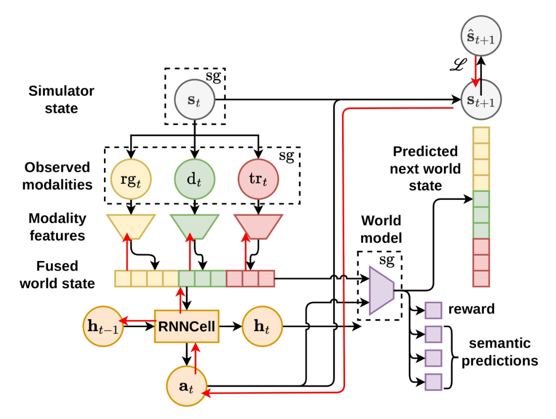
Having described the world modeling tasks, we now present a recurrent architecture that implements predictors for them.

Networks. Figure 2 shows our setup. We extract observations for each modality - roadgraph, agent locations, traffic lights, and any form of route conditioning -- and process them into a unified world state representing the current situation around the ego-vehicle. To capture temporal information, we use an RNN to evolve a hidden state according to the observed features. A world model with multiple heads predict the next unified world state, a reward, and the estimates for the three tasks introduced previously - relative odometry, state planning, and inverse state estimation.

Losses. We use four main losses - one for the control task, which drives the behavioral policy, and three additional losses for the relative odometry, state planning, and inverse state tasks. Each of these leverages the differentiability of the environment. The inputs to the world model are detached (denoted with sg[$\cdot$]) so the world modeling losses do not impact the behavioral policy. This greatly improves policy stability and makes it so one does not need to weigh the modeling losses relative to the control loss.

For extended functionality, our agent requires two additional auxiliary losses. The first trains the world model to predict the next world state in latent space, which is needed to be able to predict autoregressively arbitrarily long future sequences $\mathbf{z}_t, \mathbf{z}_{t+1}, ...$. It also allows us to use the AWM task heads on those imagined trajectories, similar to [5, 6]. The second is a reward loss so the world model can predict rewards. We use a standard reward defined as $r_t = -{\lVert \mathbf{s}_{t+1} - \hat{\mathbf{s}}_{t+1} \rVert}_2$.

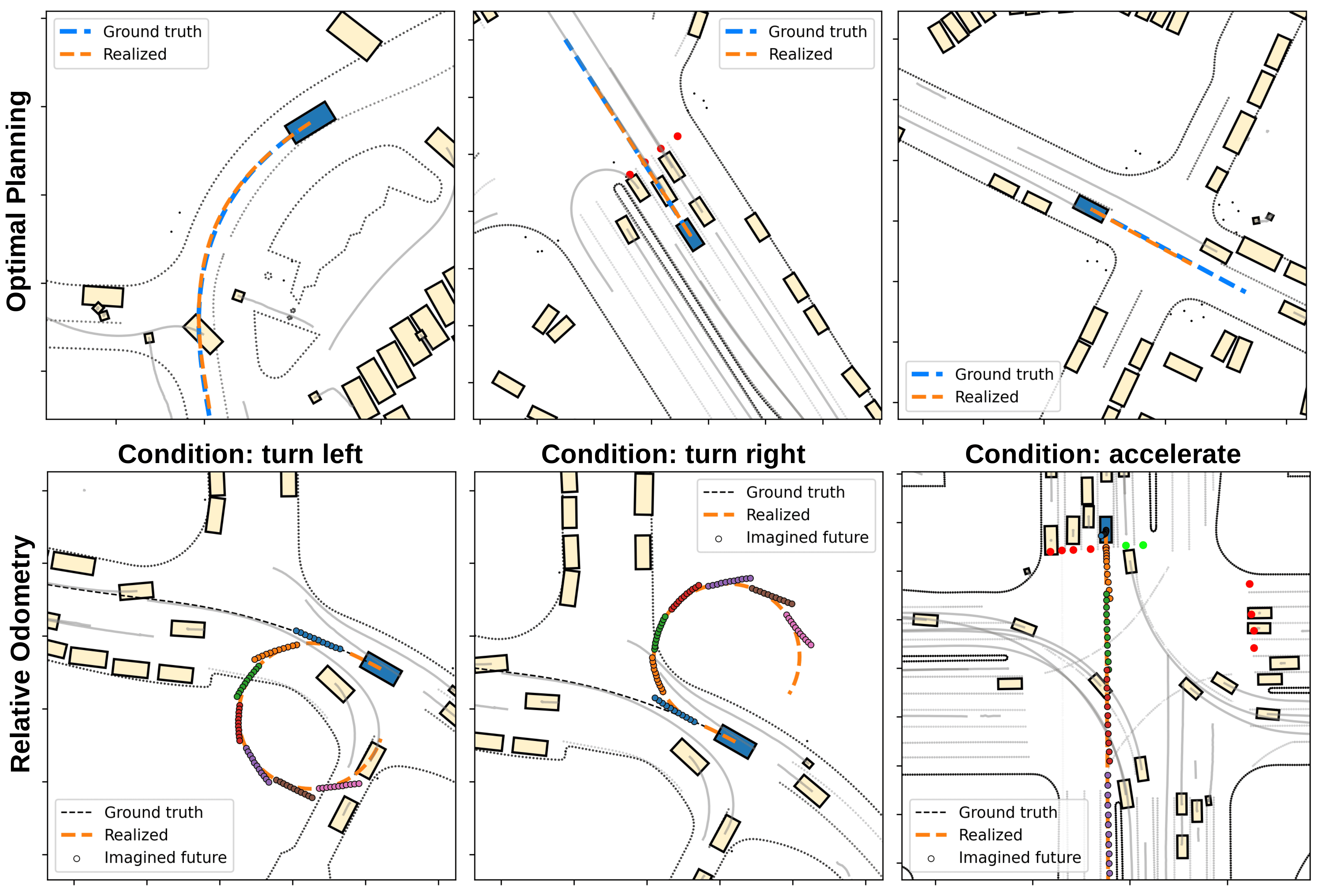
Qualitative results. Now, let's look at some quick qualitative results from the predictors. First, the top row of Figure 3 shows trajectories obtained using the planner. Specifically, the planner produces a desired next state $\mathbf{\tilde{s}}_{t+1}$ and we obtain the action $\mathbf{a}_t$ that brings us there using inverse kinematics. For good performance, if the planner is used for action selection at test time, we need set the behavioural policy at training time to also come from the planner. This is a slight nuisance, but is expected, since in general APG and AWMs work best in on-policy settings.

We can also condition the agent to steer left/right, or accelerate/decelerate. The bottom row of Fig. 3 shows predictions from the relative odometry representing the agent's own imagined motion for the next one second. Computing these trajectories is done by autoregressively rolling-out the latent world model and the odometry predictor at test time. Since the imagined trajectories align with the realized one, we judge the agent to accurately imagine its motion, conditional on a sequence of actions. The accuracy here depends on the temporal horizon and whether the action sequence is in- or out-of-distribution.

References

[1] Sutton, Richard S. Dyna, an integrated architecture for learning, planning, and reacting. ACM Sigart Bulletin 2.4 (1991): 160-163.
[2] Ha, David, and Jürgen Schmidhuber. World models. arXiv preprint arXiv:1803.10122 (2018).
[3] Gulino, Cole, et al. Waymax: An accelerated, data-driven simulator for large-scale autonomous driving research. Advances in Neural Information Processing Systems 36 (2024).
[4] Ettinger, Scott, et al. Large scale interactive motion forecasting for autonomous driving: The waymo open motion dataset. Proceedings of the IEEE/CVF International Conference on Computer Vision. 2021.
[5] Hafner, Danijar, et al. Dream to control: Learning behaviors by latent imagination. arXiv preprint arXiv:1912.01603 (2019).
[6] Wu, Philipp, et al. Daydreamer: World models for physical robot learning. Conference on robot learning. PMLR, 2023.