How To Intercept a Missile
Today, missile guidance sits at the crossroads of classical control theory, real-time signal processing and modern AI-driven state estimation. Whether you’re tuning fins on a supersonic interceptor or programming a drone swarm to shadow evasive targets, the same principles of geometry, feedback and computational efficiency govern success under extreme time pressure. Let's explore the basics of this hugely important topic.
Let's consider a simple setting. A missile is flying towards a nearby location. You want to fire an interceptor missile whose job is to hit that missile in flight, thereby preventing it from reaching its destination. We'll model the state of the target missile with its current \((x, y, z)\) position \(\mathbf{P}_t \in \mathbb{R}^3\) and velocity vector \(\mathbf{V}_t = (v_x, v_y, v_z) \in \mathbb{R}^3\). The target (ballistic) missile is gravity-affected. The interceptor missile also has a position \(\mathbf{P}_i\) and velocity \(\mathbf{V}_i\). The goal is to find a closed-loop control law for the interceptor so that the relative position \(\mathbf{R} = \mathbf{P}_t - \mathbf{P}_i\) becomes zero.
Dynamics. We'll consider some very basic continuous particle-mass dynamics with 3 degrees of freedom (DoF). The change in position is given by the velocity, \(\dot{\mathbf{P}}_t = \mathbf{V}_t\). The velocity of the ballistic missile has constant acceleration, only through gravity, \(\dot{\mathbf{V}}_t = \mathbf{g} = (0, 0, -9.8) \text{ m/s}^2\). For the interceptor, we again have \(\dot{\mathbf{P}}_i = \mathbf{V}_i\) but we'll assume it always has constant speed, \(\lVert \mathbf{V}_i \rVert = V_i\). The control variable for the interceptor is the lateral acceleration \(\mathbf{a}_i\). It affects the velocity vector \(\dot{\mathbf{V}}_i = \mathbf{a}_i\). At any point the interceptor's direction of motion is the velocity vector. Lateral acceleration is a vector drawn at 90° to that. It doesn’t add or subtract from the speed; it only bends the interceptor's path. It's like the car tires gripping and pulling you around a curve without changing your speed. We'll assume it has some maximum value, resulting in the constraints \(\mathbf{a}_i \perp \mathbf{V}_i\) and \(\lVert \mathbf{a}_i \rVert \le a_\text{max}\). The relative position of the missiles is given by \(\mathbf{R} = \mathbf{P}_t - \mathbf{P}_i\) and \(\dot{\mathbf{R}} = \mathbf{V}_t - \mathbf{V}_i\).
Proportional navigation. Next, the control law we'll use is proportional navigation guidance. The idea is that if two objects have direct line of sight (LoS) that does not change direction as their range closes, then they will collide. Intuitively, if the ballistic missile is visible at 30° yaw angle within the field of view of the interceptor, and this angle stays constant as the range between the two missiles decreases, then they will hit. If the ballistic missile moves to the right, now appearing at -30°, the interceptor will miss it, unless it turns 60° further in the same direction, so that the ballistic missile again appears at 30°. That's the basic idea. Proportional means that the change in the direction of the interceptor is proportional to the line of sight rate. Different types of controllers were covered here.
The line of sight (LoS) shows how the target "appears" in the "viewpoint" of the interceptor. More simply, it's the vector from the interceptor \(\mathbf{P}_i\) to its target \(\mathbf{P}_t\) at any instant, which is \(\mathbf{R} = \mathbf{P}_t - \mathbf{P}_i\). We want to understand its angular velocity.
Angular velocity. Let's see the angular velocity visually in Fig. 1. The vector \(\mathbf{R}\) represents a 3D point and extends from the origin \(O\). Since \(\mathbf{R}\) moves in time, it has some velocity vector \(\dot{\mathbf{R}} = (\frac{dx}{dt}, \frac{dy}{dt}, \frac{dz}{dt})\). The velocity defines the direction of motion. The vectors \(\mathbf{R}\) and \(\dot{\mathbf{R}}\) span a plane (shaded in gray) whose orientation can be found using the right-hand rule. Crucially, an angle \(\theta\) is formed between the vectors \(\mathbf{R}\) and \(\mathbf{R} + \dot{\mathbf{R}}\). The angular velocity of \(\mathbf{R}\) is a vector \(\mathbf{\omega}\) showing both the orientation of the axis of rotation through its direction - the unit vector \(\hat{\mathbf{\omega}}\) - and how fast the angle around that axis changes - through its magnitude \(\lVert \mathbf{\omega} \rVert = \frac{d \theta}{dt}\).

Here's a very intuitive interpretation. We set the origin of the coordinate system \(O\) to be the position of the interceptor. Then the vector \(\mathbf{R}\) is the target missile, as viewed from the interceptor. If the target moves radially (forward and backward) along \(\mathbf{R}\), no angle will change. Yet if it moves even a little bit off the radial direction, this will create a non-zero angle of rotation, as viewed by the interceptor. Now the math: the velocity vector \(\dot{\mathbf{R}}\) is decomposed into its radial and cross-radial components. Only the pure cross-radial rotation is of interest.
In the first line the angle is given by the arc-length divided by the radius, the radius does not depend on \(t\) because we're considering only the rotation around a fixed point. The change in the arc length is given by the length of the cross-radial part of the velocity, which can be rewritten as a cross product between the position and its velocity.
Closing speed. Next, we need the speed at which the interceptor approaches the missile. This is called the closing speed and is important because the faster you approach, the less time to you have to turn - so you need a larger lateral acceleration (in m/s²) for the same angular correction.
Control. We're ready to control the interceptor. The commanded lateral acceleration is given by
Here \(V_r\) is the closing speed, a scalar, \(N\) is the proportional coefficient, a scalar, and \(\mathbf{\omega} \times \hat{\mathbf{R}}\) is the direction of the acceleration, a vector.
- If the interceptor is closing in fast, you need larger acceleration to steer, hence the \(V_r\) term.
- The term \(\mathbf{\omega} \times \hat{\mathbf{R}}\) represents tangential velocity, i.e. the interceptor's steering direction. \(\hat{\mathbf{R}}\) is simply the unit direction of the LoS.
- The constant \(N\) tunes the aggressiveness of the pursuit. A higher \(N\) leads to tighter turns and more lead and quicker convergence. Note that the interceptor's velocity should not point exactly at \(\hat{\mathbf{R}}\), but it should lead it by some angle. If \(N=1\), the interceptor ends up on a pursuit curve, always pointing toward the current target bearing instead of “leading” it. So a higher \(N\) is usually better. Yet, increasing \(N\) increases the load - the lateral acceleration endured during turns, measured in \(g\)s. A higher \(N\) puts more structural and aerodynamic stress on the interceptor.
Thus, the general idea is to steer with a lateral acceleration proportional to how fast the target bearing is changing, and scale that by how fast you’re closing on it.
Finally, the lateral acceleration to execute is clipped to a maximal value \(a^\text{max}\):
Realism. Is it realistic to assume that we can control a missile's lateral acceleration? Well, the missile has no magic sideways thruster. In reality missiles can have very small fins or canards that generate lift when deflected, producing a side‐force. Additionally, gimbaling the main nozzle gives a thrust component perpendicular to the velocity vector. Beyond that, of course, a lot of things are missing from the mathematical formulation - actuation bandwidths and rate limits, nonlinear aerodynamic derivatives, 6-DOF rigid body dynamics, mass depletion and changing inertia as the missile's fuel runs out during its flight. Moreover, here we've assumed that the target's position is available at any time and without noise. In reality, the interceptor needs to be equipped with sensors for gathering the relevant information. Target position and velocity could be collected using seekers (e.g. radar, contrast, infrared), while its own position and velocity usually come from INS and possibly GPS. Finally, to deal with sensor noise things like the extended Kalman filter are used.
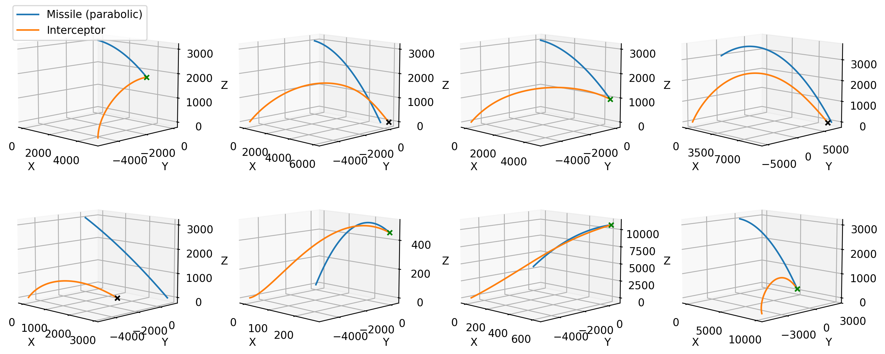
Simulation. Fig. 2 shows different cases where we've discretized the control law and the dynamics to simulate the trajectories. The target missile is in blue and the interceptor, always starting from the ground level, is in orange. Reaching the target happens if the distance between the two missiles is below 10 meters. This event is marked with a green cross, while not reaching is black. If any of the missiles hit ground level, their trajectories end. Notice how in some cases the interceptor successfully reaches the target, while in others it fails, it heavily depends on the starting positions and the slope of the target's trajectory. A higher proportionality constant usually helps - e.g. first row second plot uses \(N=3\) while first row third plot uses \(N=5\).
You can see that missile interception is a very important topic because additional optimizations and more sophisticated machinery could literally save lives. We've barely scratched the surface here. What happens if in addition to interception, we want to minimize the interceptor's flight time, or we want to minimize some kinematic constraints on the flight? What if the target missile is programmed to make false jagged moves to mess with the interceptor? What if there are multiple missiles and there are only a few interceptors? Which ones should be prioritized? People have devoted their careers to this, as well as entire industries have sprung up around these problems. In game theory similar pursuit-evasion games have been studied extensively. It's really one of those fascinating applications of math, cs, and engineering that are of critical importance in some situations, yet you will wish these situations occur as infrequently as possible.