Impulses, Feedback, Control
Control engineering is a very useful topic for the real world. It is concerned with studying dynamic systems and figuring out how to control them in a way that is beneficial for us. I've encountered multiple references to it but have never studied it carefully. In autonomous driving, for example, it's common to predict a bunch of waypoints marking the intended future trajectory of the vehicle. You then give them to a PID controller that will try its best to follow that trajectory. But how does it work exactly? Well, I'm quite satisfied that I finally got to read up a bit on this topic. Because the principles of control theory are applicable in diverse contexts - reinforcement learning with known dynamics, economic policy design, digital filters for audio and image processing, everywhere really.
Consider a one-dimensional dynamic system which depends on some continuous control input variable \(u(t)\) and produces some measurement variable \(x(t)\). The exact relationship between \(u(t)\) and \(x(t)\) could be complicated and is typically modeled using differential equations. As an example, a mass \(m\) attached to a damper with damping coefficient \(b\) could be modeled as
where time derivatives are denoted with dots. If we start at \(x(0) = 0\) and "bump" the system by giving it a single instantaneous Dirac unit spike \(u(t) = \delta(0)\) applied at \(t=0\), instead of an immediate jump in position \(x(t)\), the system converts the spike into an immediate jump in velocity, which gradually moves the position \(x(t)\), converging to \(1/b\). It acts as a low-pass filter absorbing sudden changes via damping. A sudden change in \(u(t)\) causes a gradual change in \(x(t)\).
Goal. The general task of control theory is to choose a function \(u(t)\) such that the system output \(x(t)\) follows some desired behaviour, could be tracking a reference trajectory \(r(t)\), regulation to fixed value \(x(t) \rightarrow a\), or minimizing some cost function over \(x(t)\). All of these require studying how the control \(u(t)\) affects the output \(x(t)\) and have many exciting applications - fusion plasma stabilization, autonomous aerospace guidance, cruise control, TCP congestion control, legged-robot balancing, closed-loop neuromodulation, etc.
Laplace transform. The way to study these systems is in the complex frequency domain, called the \(s\)-domain, through the Laplace transform. It takes a real function of time \(f(t)\) and converts it to a complex-valued function \(F(s)\) with \(s = \sigma + j \omega\):
The transform is defined only for those \(s\) for which the exponential \(e^{-st}\) decays fast enough to counteract any growth in \(f(t)\), so the integral can be finite. The benefit of the Laplace transform is that it turns differentiation (and integration) in the time domain into multiplication (and division) in the \(s\)-domain. To see this, we integrate by parts:
Here, functions in the \(s\)-domain are indicated in capital. Unfortunately, the Laplace transform of a derivative represents the initial condition explicitly through the additive term \(-f(0)\). It is common to assume that our control systems starts from \(0\), so that \(f(0) = 0\) and \(\mathcal{L}[\dot{f}(t)] = sF(s)\). When making this assumption we're effectively only analyzing the forced response of the system (what output will be provoked by the input), not its natural response (containing initial energy decay).
LTI systems. Now, if our control system \(\dot{y}(t) = f(y, u)\) is linear and time-invariant, abbreviated LTI, its representation in the \(s\)-domain has a particularly simple multiplicative form, \(Y(s) = H(s) U(s)\). Here time-invariant means that the behaviour does not depend on the particular moment in time. There are no terms like \(u(t)t\) or non-constant coefficients like \(g(t)\dot{y}(t)\). Linear means that the mapping from control inputs to outputs obeys superposition. If \(u_1(t)\) produces \(x_1(t)\) and \(u_2(t)\) produces \(x_2(t)\) then \(au_1(t) + bu_2(t)\) produces \(ax_1(t) + bx_2(t)\). Any nonlinear terms like \(x(t)^2\) or \(x(t)u(t)\) would prevent this.
For example, the system \(\beta \dot{y}(t) + y(t) = Ku(t)\) is LTI. Assuming \(y(0)=0\) for simplicity, we apply the Laplace transform on both sides of the equation and rearrange to get:
Transfer function. The term \(H(s)\), here equal to \(K/(\beta s + 1)\), is called the transfer function and characterizes the behaviour of the system. It's simply defined as the \(s\)-domain ratio of the output over the input of a LTI system, \(H(s) = Y(s)/U(s)\). Studying the transfer function can yield precious information about the system's dynamics and stability. Note that if we model some system as \(Y(s) = H(s)U(s)\) we're assuming that \(y(t)\) is LTI. A non-LTI system simply cannot be represented as a multiplication in the \(s\)-domain. For the same reason the transfer function is only meaningfully defined for LTI systems.
Impulse response. By definition the Laplace transform of a single Dirac delta is \(1\). Therefore if we feed the system a single Dirac delta, it will respond in the \(s\)-domain with its transfer function. Thus, the impulse response \(h(t)\) in the time domain is the inverse Laplace transform of the transfer function \(H(s)\). Similarly, the transfer function is the Laplace transform of the impulse response. The impulse response characterizes the behavior of the system. Any input signal \(u(t)\) can be represented as a superposition of multiple scaled impulses. The output \(y(t)\) is then, by linearity, a superposition of impulse responses, weighed by the control \(u(\cdot)\):
The impulse response of our simple system is \(h(t) = \frac{K}{\beta}e^{-t/\beta}, \ t \ge 0\). Here we manually restrict the domain to \(t\ge 0\) so the system is causal. There is no response before the input impulse happens. Thus, an instantaneous spike in the controls at \(t=0\) causes an immediate jump to \(K/\beta\) and an exponentially fast subsequent decline to \(0\). Given a control signal \(u(t)\) the output is
If \(\beta\) is large, the impulse response decays slowly and past controls before \(t\) greatly affect \(y(t)\). Otherwise, only the most recent \(u(t)\) close to \(t\) affect \(y(t)\).
Frequency response. Similar to input impulses, we can ask what the output will be if we are providing a continuous sinusoid of constant frequency as input. Now, a general property of LTI systems is that if the input is a complex sinusoid, the output is always also a scaled/shifted complex sinusoid. Thus, \(e^{st}\) is an eigenfunction and \(H(s)\) is the eigenvalue. To verify, consider the input \(u(t) = e^{st}\). The output is:
Remember that \(s = \sigma + j\omega\). Hence \(e^{st} = e^{\sigma t} e^{j \omega t} = e^{\sigma t}(\cos \omega t + i \sin \omega t\) is a decaying/diverging sinusoid. For a normal sinusoid we set \(\sigma=0\) and obtain \(y(t) = H(j\omega) e^{j \omega t}\). The quantity \(H(j\omega)\) is the frequency response and is given simply by \(H(j\omega) = \left. H(s) \right\vert_{s = j\omega}\).
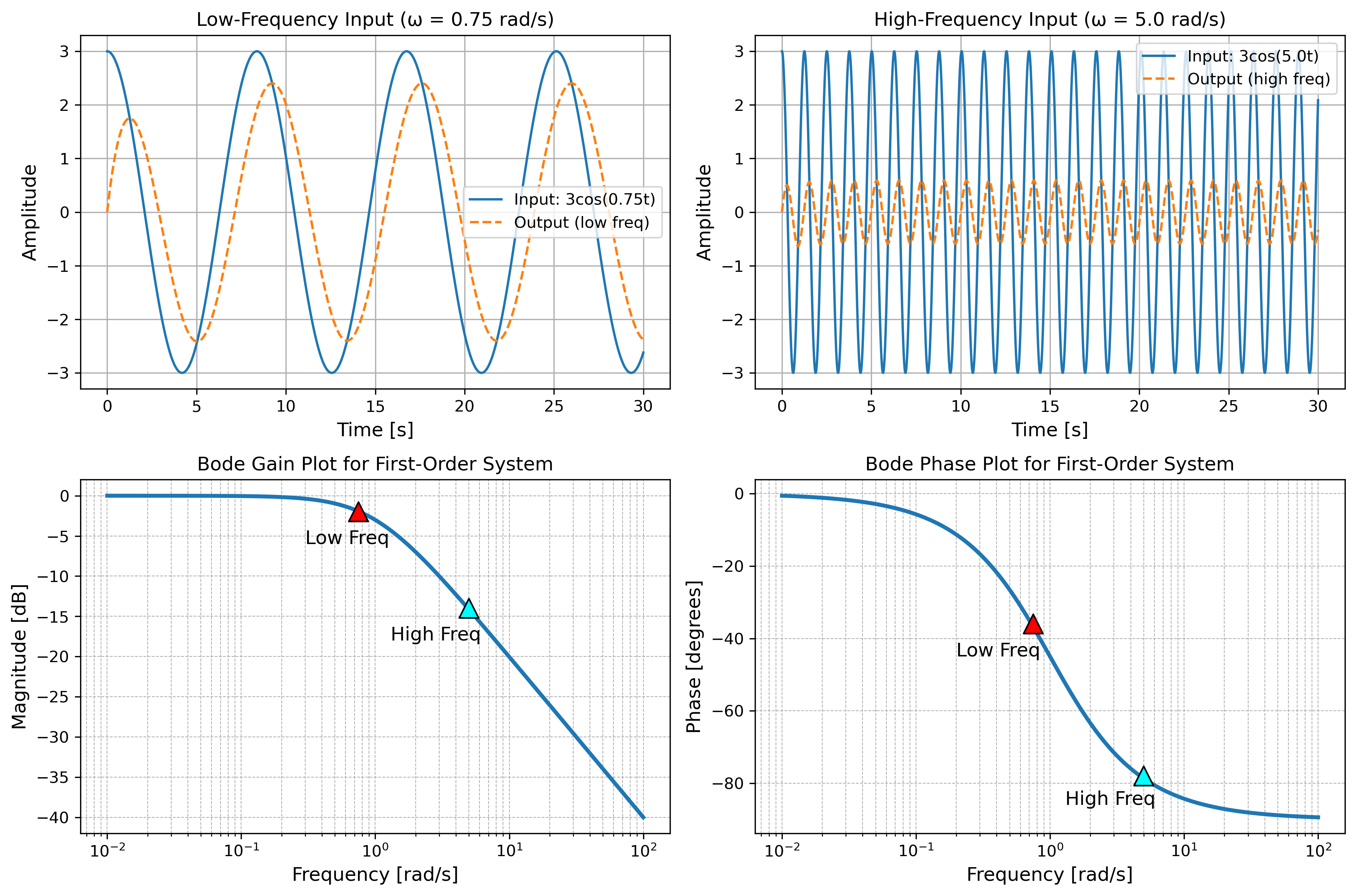
For our system the frequency response is \(H(j\omega) = K/(1 + j \omega \tau)\). This is a complex number, depending on the input frequency \(\omega\). We can compute the magnitude and phase
Here's what happens, at small frequencies the magnitude, called gain, becomes \(K\), while the phase is \(0\). Therefore, at low frequencies the output signal is scaled by \(K\) and has virtually no phase lag. At larger frequencies \(\omega\), the gain magnitude scales as \(K/(\beta \omega)\). In log-terms, for each tenfold increase in \(\omega\), the magnitude drops by \(20 \log_{10}(10) = 20 \text{dB}\). This is "-20 dB/decade". For very large \(\omega\), it becomes \(0\) and the phase difference is \(-90\) degrees, lagging by about a quarter period. Importantly, the frequency response shows how the input sinusoid is amplified and lagged only in the steady state, after any transient dynamics have faded.
Poles and zeros. The transfer function describes the behavior of the system in complex frequency space. Consider the points at which it is equal to zero. These are the roots of the numerator of the transfer function and are conveniently called zeros. Likewise, the roots of the denominator are the points at which the transfer function is infinite in magnitude, they are called poles. Each pole \(s_p\) contributes a \(\exp(-s_p t)\) term in the time-domain of the solution. Hence, all stable systems, those whose responses do not eventually blow up to infinity, need the real part of all their poles to be negative. If a pole is positive, its response term is exponentially increasing in time.
A pole at \(s=0\) is called an integrator because the resulting output is \(y(t) = \int_{0}^t u(\tau) d \tau\). In that sense, if we apply a constant control of \(1\) for, say, \(3\) seconds, the output will be \(3\). Such an integrator is said to have perfect memory because it never forgets previous inputs, they all contribute to the current output. A bounded input like a step produces an unbounded ramp.
Sometimes poles come as complex conjugate pairs \(\sigma \pm j \omega_d\). Their contributed terms \(e^{(\sigma \pm j \omega_d)t}\) are thus sinusoidal oscillations which decay in \(t\) when \(\sigma < 0\) or diverge when \(\sigma > 0\). For example the transfer function \(H(s) = 1/(s^2 + s + 1)\) has poles at \(-1/2 \pm j \sqrt{3}/2\). Its impulse response is given by \(h(t) = \frac{2}{\sqrt{3}} e^{-t/2} \sin(\frac{\sqrt{3}}{2}t), t \ge 0\). Hence, it "rings" at \(\frac{\sqrt{3}}{2}\) rad/s with an \(e^{-t/2}\) envelope.
Open-loop control. Now, let's move to the question of how to actually control the system so that it produces a desired reference signal \(r(t)\). One idea, called open-loop is the following. The system output in the \(s\)-domain is \(Y(s) = H(s)U(s)\). The controller \(c(t)\) and similarly \(C(s)\) is a function which selects the controls so that it best follows the reference \(r(t)\) or \(R(s)\). Assuming that \(H(s)\) is invertible (which is often more than we can ask), we can take \(C(s) = H(s)^{-1}\). Then, we input the desired reference trajectory \(R(s)\) into the controller, which produces the controls \(H(s)^{-1} R(s)\). This goes into the system and produces \(Y(s) = H(s) H(s)^{-1} R(s) = R(s)\).
This kind of control is basically feedforward via model inversion, it's simple but fragile. Oftentimes exact inversion is numerically unstable. However, a bigger problem is that there is no way to correct the controls you set. Therefore, small errors made earlier could accumulate into large errors later on. For this reason, we need something more adaptive.
Closed-loop control. Here the idea is that we'll incorporate feedback. The controller will now take as input the error \(r(t) - y(t)\) when outputting \(u(t)\). In that sense we're closing the loop, because now \(r(t) - y(t)\) leads to \(u(t)\), which leads to \(y(t)\), which leads to a new \(r(t) - y(t)\) and so on. The controller takes in \(R(s) - Y(s)\) and its output is \(C(s)[R(s) - Y(s)]\). This goes through the system producing \(H(s) C(s) [R(s) - Y(s)]\), which is equal to the actual output \(Y(s)\). Hence:
Here \(T(s)\) is the transfer function of the entire system with the closed loop controller baked in. Note that stability is guaranteed when the poles of \(1 + H(s)C(s)\) all have negative real parts. Computing the poles however, can be quite difficult. There are various criterions (e.g Routh–Hurwitz, root locus, Nyquist) which can be used to qualitatively inspect the behaviour of the poles.
Proportional controller. So what should \(C(s)\) be? In the simplest setting, it's just a constant, \(C(s) = K_p\). With a constant trasnfer function, the output in the time domain is \(u(t) = (c \ast e)(t) = \int_{0}^\inf K_p \delta(\tau)e(t - \tau) d\tau = K_p e(t)\), where \(e(t) = r(t) - y(t)\). Thus, the constant \(K_p\) simply scales the error term. \(K_p\) has to be tuned so the response tracks \(r(t)\) accurately and without overshooting.
PI controller. This controller is given by \(C(s) = K_p + K_i/s\). Here, \(K_p\) scales the error as before but there is an integrator (the I in the name) \(K_i/s\). This means that if, for whatever reason, \(y(t)\) is consistently larger than \(r(t)\), the integral of the error will start to become bigger and bigger. Eventually, it will overlwhelm any other error terms, e.g. the \(K_p e(t)\), and it will cause the controller to prioritize decreasing \(y(t)\) below \(r(t)\). This is very useful if the controls are biased in that they stay above or below the reference for extended time.
PID controller. This last improvement changes the controller transfer function to \(C(s) = K_p + K_i/s + K_d s\) by introducing a term \(K_d s\). In the time domain this looks like \(K_d \frac{d}{dt}e(t)\). This new term adds damping: it makes the denominator of \(T(s)\) resist rapid changes in error, similar to how a shock absorber resists quick motion tames oscillations. The time-domain formulation for the PID is:
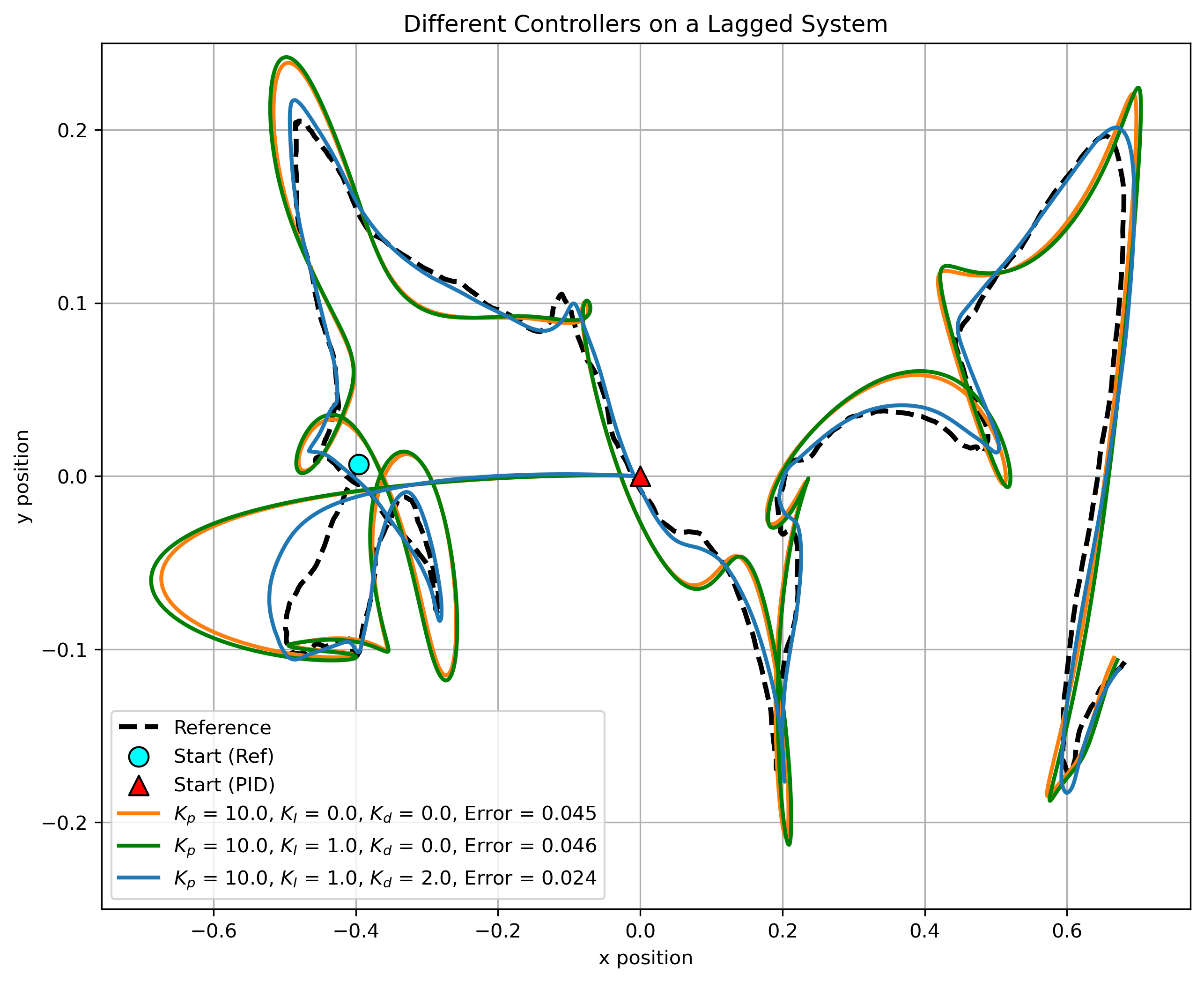
Figure 2 shows a very simple simulation where we're tracking a reference trajectory (dashed black) with the three controllers. The equations of motion represent a first-order lag system where the control \(u_x\) affects the velocity \(v_x\) as \(\dot{v}_x = (u_x - v_x)/\tau\). Then, the derivative of the \(x\)-position is \(\dot{x} = v_x\). The same motion is used also for the \(y\)-coordinates. These dynamics are sufficiently complicated to demonstrate that a PID controller performs better than a P or PI controller. Note how the reference and the controllers start from quite different points. The controllers have to quickly catch up to the reference.