The Phase Stretch Transform | The Critical Section

I have recently discovered PhyCV - an awesome new physics-inspired computer vision library. It contains refreshing new algorithms for various imaging tasks, all of them with a physical justification [1]. This post explores one of these - the phase stretch transform (PST), which can be used to detect edges and corners, or enhance even the faintest visual features in images from poorly-lit environments. It's a very clever technique and getting to know how it works also yields, as a benefit, some basic knowledge in topics like Fourier optics and wave propagation.

In general, the phase stretch transform builds on top of other ideas which one should understand. The most basic of these is the notion of a wave - a disturbance that is being propagated through space and time in a given medium. There are many types of waves - acoustic waves, mechanical waves and electromagnetic waves being a few of them. One of the simplest waves is the sine wave, modelled as

$$ \Psi(x, t) = A \sin (k x - \omega t + \phi). $$

Here $x$ is a spatial one-dimensional variable and $t$ is a temporal variable. $A$ is called the amplitude of the wave and shows how far a given quantity is from its equilibrium. In the case of acoustic waves, this would be air pressure. In the case of water waves (a type of mechanical waves) the amplitude may be the current height of the wave, as measured from the average. In general the magnitude may depend on the position $(x, t)$. Everything within the sine function is called the phase and affects the spatio-temporal positioning of the wave. The parameter $k$ is the wavenumber - a measure of the spatial frequency - and $\omega$ is the temporal frequency affecting how fast the wave at a fixed space position repeats in time. $\phi$ is called the phase shift because it further shifts the wave without changing its spatial or temporal frequencies.

It is useful to represent waves mathematically using complex numbers:

$$ \Psi(x, t) = A e^{i(kx - \omega t + \phi)} = A \cos(kx - \omega t + \phi) + i A \sin(kx - \omega t + \phi). $$

For a wave with fixed parameters $(k, \omega, \phi)$ evaluating it at a position $(x, t)$ requires two numbers, the amplitude and the phase, and conveniently, these can be represented as a single complex number. As per Euler's formula, the complex exponential form is just a more convenient way to represent the sum of a cosine and a complex sine. Additionally, transforming the point $(A\cos(kx - \omega t + \phi), A\sin(kx - \omega t + \phi))$ from Cartesian to polar coordinates yields exactly the amplitude and the phase $(A, kx-\omega t + \phi)$. Note that the real component of the wave value serves to model actual observable quantities from the real world. The fact that it comes from a cosine is not problematic because the cosine function is just a phase-shifted sine.

Various signals like audio samples or images can be considered as a superposition of many individual waves. And the Fourier transform, a tool that is ubiquitous in signal processing, can be used to disentangle the aggregate signal into its individual constituents. In that context, it is a very important insight that phases tend to carry more of the "useful" information, compared to amplitudes. This can be visualized easily using the two-dimensional Fourier transform applied on images.

Applying the 2D FFT on images works as follows. If the image is single-channel, with size $(H, W)$, we assume the spatial sampling frequency is $1.0$ and therefore by Nyquist the maximum spatial frequency we can capture is $0.5$. So the frequency bins for the height are $H$, spread linearly from $-0.5$ to $0.5$. Similarly, those for the width are $W$, spread from $-0.5$ to $0.5$. The FTT shows, for two particular frequency bins along the image axes, how much of them is present in the image.

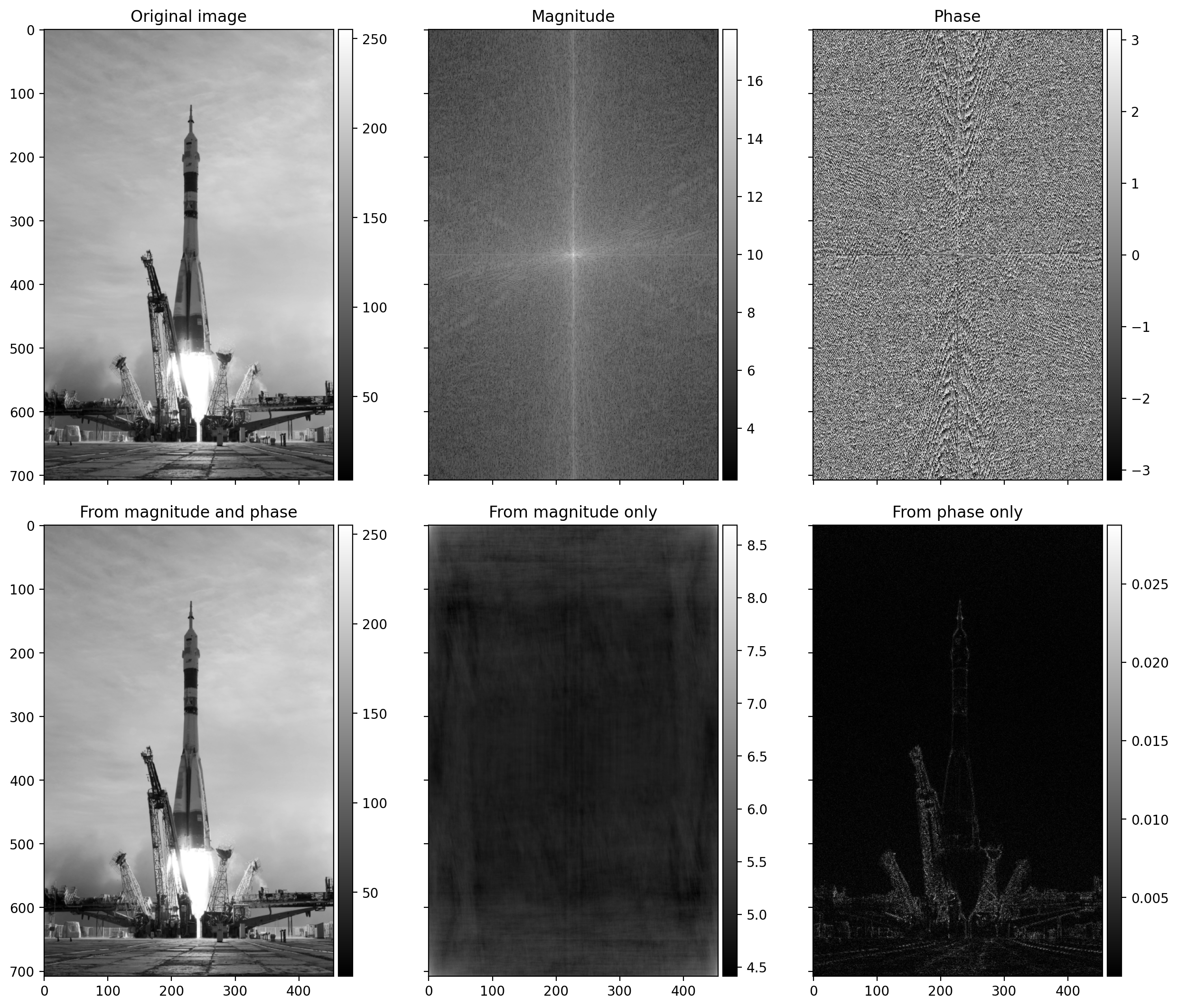
Figure 1 shows a classic experiment where we take the two-dimensional Fourier transform of one image, and reconstruct it with either the magnitude, or the phase, or both. In essence, the Fourier transform outputs a dense matrix of complex numbers. Their magnitudes, $\sqrt{x^2 + y^2}$, and phase angles, $\tan^{-1}(y/x)$, are plotted for visualization. The plot of the magnitudes is commonly called the Fourier spectrum. Applying the inverse 2D FFT on the magnitudes only produces an almost entirely dark image, whereas reconstructing from the phases produces the main contours of the objects from the original image.

Fourier reconstructions — Figure 1: Various outputs from the Fourier transform. The input image is in the top left. The second and third images contains the magnitude and phase from the Fourier transform. The second row contains reconstructions using the inverse Fourier transform. The magnitude images have been log-scaled for visual clarity. When reconstructing from phases only, the absolute value of the real components are plotted for better contrast.

Reconstructing with the actual magnitudes and a set of random phases, or with the actual phases and a set of random magnitudes does not change the output noticeably. Or even mixing the magnitudes and phases of two different images will produce a blurry image with visible contours coming from the image from which the phases were taken. All of this shows that for visual signals, where most of human perception is based on edges, corners and contours, the phases of the waves are more important than the magnitudes.

This is the first hint that by modifying the phases we can change the shapes of the objects in the image and potentially enhance any edges or visually impaired features.

Moving on, we now consider how waves can form superpositions. This is useful when dealing with the phase stretch transform. Suppose we have two cosine waves with only slightly different spatial and temporal frequencies:

$$ \Psi_A(x, t) = A \cos(k_1 x - \omega_1 t + \phi) \\ \Psi_B(x, t) = A \cos(k_2 x - \omega_2 t + \phi). $$

Using a trigonometric identity we can express their sum as

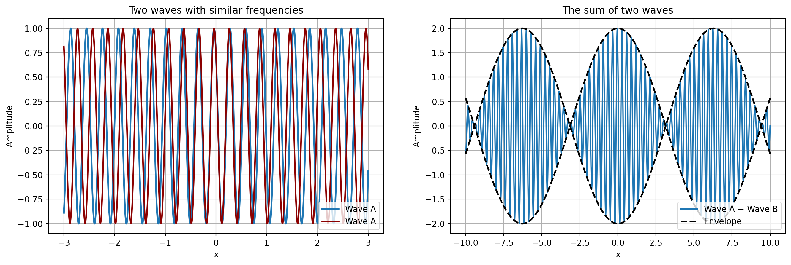
$$ \begin{align} \Psi_{A + B} = & A \cos(k_1 x - \omega_1 t + \phi) + A \cos(k_2 x - \omega_2 t + \phi) \\ = & 2 A \cos \big (\frac{k_1 - k_2}{2}x - \frac{\omega_1 - \omega_2}{2}t \big ) \cos \big ( \frac{k_1 + k_2}{2}x - \frac{\omega_1 + \omega_2}{2}t + \phi \big ) \end{align} $$

As can be seen from Figure 2 the aggregate wave has a complicated shape. The component $2 A \cos \big (\frac{k_1 - k_2}{2}x - \frac{\omega_1 - \omega_2}{2}t \big )$ is called the envelope because it tightly surrounds the aggregate wave at any point $(x, t)$. The other, higher-frequency wave is called the carrier wave (or sometimes the ripples) because it carries the useful signal of the envelope and is being modulated by it.

If we release a small object into a current flowing like the waves here, we can measure two different velocities - the phase velocity and the group velocity. The phase velocity is the velocity (in meters per second or any other units) with which any particular frequency component of the wave travels. It is given by $\nu_p = \omega / k$ - angular change per unit of time divided by angular change per unit of space. In contrast, the group velocity is the velocity with which the envelope of the wave propagates through space, and is given by $\nu_g = \partial \omega / \partial k$ (in the continuous case).

The waves discussed here are unrealistic because they extend infinitely in time and space. In reality, many waves are localized - their amplitudes are non-zero only in some region of space, and decay to zero outside of that region. These waves are called wave packets or impulses because they are a superposition of many (potentially infinite) monochromatic waves which add up constructively in a given region and cancel out anywhere else. This is what makes a wave packet localized.

We can construct such wave packets using infinitely many individual single-frequency waves in a way similar to the Fourier series. If we start with an initial wave space profile of $\Psi(x, t=0) = \Psi(x)$, we are interested in what $\Psi(x, t)$ is for a general $t$, i.e. how the wave packet evolves. Skipping the derivation, our general wave packet is given by

$$ \begin{aligned} \Psi(x, t) & = \frac{1}{\sqrt{2 \pi}} \int_\infty^\infty g(k) e^{i(kx - \omega(k) t)} dk \\ g(k) & = \frac{1}{\sqrt{2 \pi }} \int_\infty^\infty \Psi(x, 0) e^{-i k x} dx \\ \end{aligned} $$

This is pretty intuitive. We take the Fourier transform of the initial wave at time $t=0$ to obtain the power of the frequencies indexed by $k$. Then for each of them, we have a wave with amplitude $g(k)$ and phase $kx - \omega(k) t$. Note that what exactly $\omega(k)$ looks like depends on how the wave packet interacts with the medium. Specific wave equations will yield different $\omega(k)$.

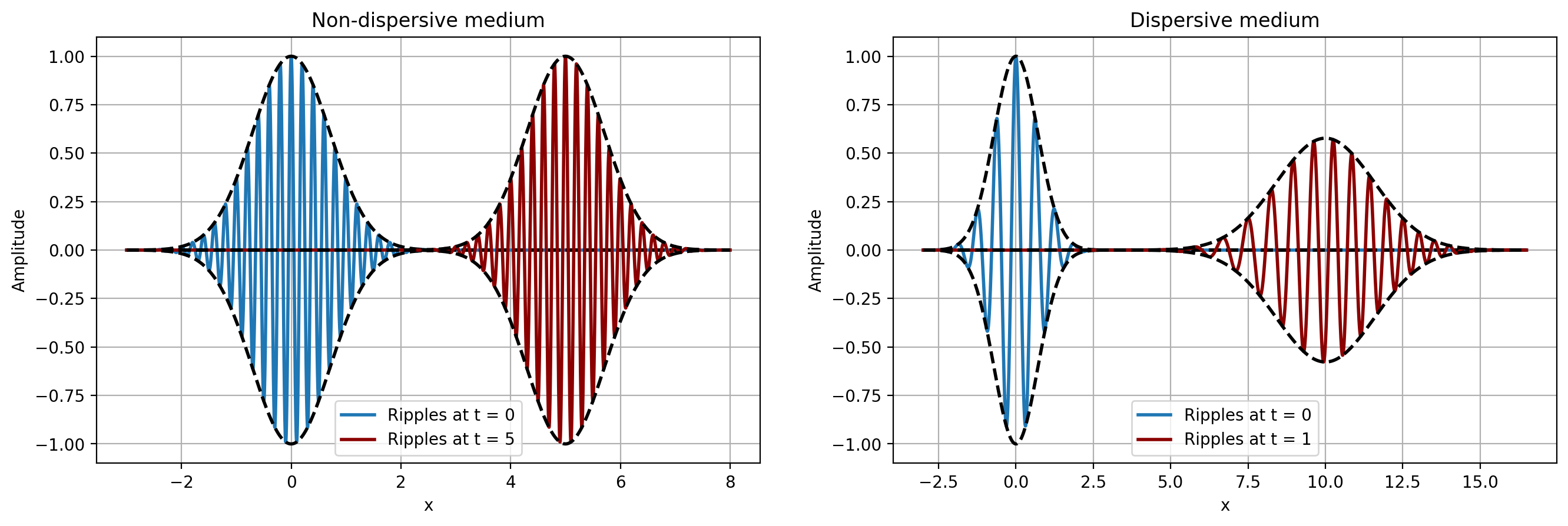
In vacuum, an electromagnetic wave has a constant $\omega$, independent of $k$. This means that all monochromatic waves travel at the same speed and as a result, the phase velocity is equal to the group velocity. The envelope travels as fast as the individual waves and its shape is constant. This is not the case in some specific mediums, for example optical fiber, where individual waves have different phase velocities. What happens to the envelope of a wave packet if some waves travel faster than others? The envelope "shapeshifts" - it gets stretched or squished. This is called dispersion.

Additional insights can be gained by exploring how an electromagnetic pulse, like light, propagates in a dispersive medium, like a fiber. This will be useful to showcase how optical dispersion in fiber changes the phases of the waves. Wave propagation is a complicated topic and the cornerstone here is the following partial differential equation:

$$ i \frac{\partial A }{\partial z} + \frac{i \alpha}{2} A - \frac{\beta_2 }{2} \frac{\partial^2 A}{\partial t^2 } + \gamma |A|^2 A = 0. $$

This equation is fundamental and deserves some explanation:

We can imagine a one-dimensional horizontal fiber of length $L$. The variable $z$ is the spatial distance from the start of the fiber, and ranges from $0$ to $L$. The variable $t$ is the time and shows how various quantities change through time.
Suppose the input signal is $f(t)$. As it travels through the fiber it's modified by various fiber characteristic effects into the output signal $y(t)$. Our main interest is in estimating what is $y(t)$ and how $f(t)$ changes into it.
$A(z, t)$ is the amplitude of the envelope at position $z$ and time $t$.
$\alpha$ is an attenuation parameter and is related to how much information is lost in the fiber. The entire term $i \alpha A /2$ represents the loss at the current amplitude.
$\beta_2$ is called the group velocity dispersion (GVD) parameter. It relates to how the pulse travelling through the fiber broadens due to dispersion. This happens because in a dispersive medium the phase velocity of individual monochromatic waves depends on the wavelength and hence the shape of the pulse, itself being a combination of possibly many waves, is broadened as some of the waves start to travel faster than the pulse itself.
The $\gamma$ parameter controls the nonlinearity term $\gamma\|A\|^2 A$ and represents the Kerr effect, one of many nonlinear effects that could arise in optical fibers. These are mainly caused by the fact that the polarization density depends nonlinearly on the electric field of the light.

It's worth mentioning that if $\alpha = 0$ we get the Nonlinear Schrödinger Equation (NLSE), where the role of the spatial and temporal variables have been swapped. In general, the pulse propagation equation does not have a close-form analytical solution. In practice it's solved numerically using finite differences or the so-called Split-step Fourier method which is at least an order of magnitude faster.

To understand the phase stretch transform we have to solve the pulse propagation equation. However, we'll simplify considerably by assuming that the fiber is lossless, $\alpha = 0$, and that there are no nonlinearities. This leaves only the dispersion term and makes the resulting equation resemble the heat equation in functional form:

$$ \frac{\partial A}{\partial z} = - i \frac{\beta_2}{2} \frac{\partial^2 A}{\partial t}. $$

The shortest solution is to transform both sides of the equality into frequency space and solve the equation there. For simplicity, let's consider this Fourier transform form (other conventions are also possible) $ \tilde{f}(\omega) = \int_{-\infty}^\infty f(x) e^{-i\omega x} dx$ and $ f(x) = (2\pi)^{-1}\int_{-\infty}^\infty \tilde{f}(\omega) e^{i\omega x} d\omega.$

$A$ consists of two variables, $z$ and $t$. We apply the Fourier transform along the $t$ dimension, after which we get

$$ \frac{\partial }{\partial z}\tilde{A}(z, \omega) = -(i \omega)^2 i \frac{\beta_2}{2} \tilde{A}(z, \omega) = i \omega^2 \frac{\beta_2}{2} \tilde{A}(z, \omega). $$

Here $\tilde{A}(z, \omega)$ is the transformed amplitude and $\omega$ is the angular frequency. The equalities above hold due to the derivative property of the Fourier transform. In any case, we can solve this ODE, and use the transformed boundary condition $\tilde{A}(0, \omega) = \tilde{f}(\omega)$ to obtain a solution in the frequency domain

$$ \tilde{A}(z, \omega) = \tilde{f}(\omega) e^{i \frac{\beta_2}{2} z \omega^2}. $$

The general solution then uses the inverse Fourier transform and is

$$ A(z, t) = \frac{1}{2 \pi} \int_{\infty}^\infty \tilde{f}(\omega ) e^{i \frac{\beta_2}{2} z \omega^2} e^{i \omega t} d\omega $$

By setting $z = L$ we obtain the output signal at the end of the fiber:

$$ y(t) = \frac{1}{2 \pi} \int_{-\infty}^\infty \tilde{f}(\omega) e^{i \frac{\beta_2}{2} L \omega^2} e^{i \omega t} d\omega. $$

This shows that in a dispersive lossless fiber medium with no nonlinearities the output signal is essentially the same, except that it is modified in frequency space by the term $\exp (i \beta_2 L \omega^2 /2 )$ which results from the dispersion. Since multiplication by complex exponentials changes the phases of the waves, what happens is that the dispersive fiber warps the signal and its contents. This happens by changing the phases of the original input function $f(t)$ in the frequency domain. Note that the amplitude is not changed.

At this point, we can change the complex exponential term (equal to the system's transfer function) to do something useful. In images, this would be for example to enhance any present edges by adding additional phase to those frequencies which are high, as edges tend to have higher spatial frequency. Additionally, although the solution above does not change the amplitude, in practice it makes sense to do so in the form of a low-pass filter. Its necessity stems from the possibility that any noise in the image may also get enhanced from the phase-addition operation and hence, to avoid this, it may be useful to blur the image first. Based on this, one can define the time stretch operation as

$$ \mathbb{S}\{ f(t) \} = \int_{-\infty}^\infty \mathcal{F}\{f(t)\} e^{i \phi(\omega)} \tilde{L}(\omega) e^{i \omega t} d \omega. $$

Here $\mathcal{F}$ is the one-dimensional Fourier transform mapping the original input signal $f(t)$ from time domain to frequency domain $\tilde{f}(\omega)$, $\tilde{L}(\omega)$ is the low-pass filter which in the frequency domain is a multiplication, and $e^{i \phi(\omega)}$ is the phase filter that serves to stretch the phases based on their frequencies. It is called a time stetching operation because by changing the phases of the individual waves making up the wave packet we are stretching or squishing its envelope in time. In fact, this has found incredible applications [2].

Finally, with images we do not have any time and any frequencies present are spatial. Additionally, digital images are inherently discrete. Based on these two observations one can define the phase stretch transform (PST), which is basically the two-dimensional, discrete spatial version of the previous operation:

$$ \mathbb{S}\{ E_i[n, m]\} = \frac{1}{MN} \sum_{v = 0}^{N-1} \sum_{u = 0}^{M-1} \text{FFT}^2 \{ E_i(n, m) \} \tilde{K}(u, v) \tilde{L}(u, v) e^{i \frac{2 \pi}{M} um} e^{i \frac{2 \pi}{N } vn }, \\ \text{PST}\{E_i[n, m]\} = \measuredangle \mathbb{S}\{E_i[n, m] \}. $$

So the stretching operation applies a phase filter $\tilde{K}$ and a low-pass filter $\tilde{L}$ in the frequency domain, returning a complex number for every combination of pixel coordinates $n$ and $m$. The PST in that location is simply the phase, or angle with respect to the real axis, of that complex number. At this point the edges, corners, and features have been enhanced. We can further normalize the phases so they're in the range $[0, 1]$ or apply morphological operations in order to:

Set the pixels corresponding to non-edges to 0 using thresholding,
Thin out or thicken the edges using erosion/dilation techniques.

The most important thing not discussed so far is what the phase kernel $\tilde{K}(u, v)$ looks like. It has to change the phase, so it has the form of $e^{i \phi(u, v)}$, but for the actual function $\phi(u, v)$ there are many possibilities. We want to add more phase to those points with large frequencies $u$ and $v$, so it's sensible to have a univariate function based on the magnitude $r = \sqrt{u^2 + v^2}$. So we need to specify the function $\phi(r)$, operating in polar coordinates. The authors of the phase stretch transform propose the following function:

$$ \phi(r) = S \frac{Wr \arctan (Wr) - 0.5 \log (1 + (Wr)^2 )}{Wr_{max} \arctan (Wr_{max}) - 0.5 \log ( 1 + (Wr_{max})^2)}. $$

Let's unpack. The function $x \arctan x - 0.5 \log(1 + x^2)$ is the integral of the $\arctan$ function. Why do we care about that? Because it's useful for $\phi(r)$ to have a linear or sublinear derivative and the $\arctan$ function is linear around 0 and sublinear (flattens out) far from it. At this point I have searched quite a lot on why exactly it makes sense to have $\phi$ have at most linear derivatives, but none of the authors, in any of the papers give a satisfactory explanation for this. In signal processing, it's useful for a filter to change the phase of the input signal in a linear way with respect to the frequency, which leads to a constant delay of the output signal and no distortion. Here, however the linear phase derivative seems hard to interpret intuitively.

In any case, there is a parameter $r_{max}$ which is the maximum magnitude of the frequencies in polar coordinates and $S$ and $W$ are edge-detection hyperparameters. Specifically, $S$ is called the strength parameter because it affects the overall range of the phase kernel $\phi$. $W$ is called the warp parameter because it affects the curvature of the phase derivative:

If $W \rightarrow 0$, the phase derivative becomes linear and the phase kernel $\phi(r)$ becomes quadratic
If $W \rightarrow \infty$, the phase derivative flattens out and is bounded, and $\phi(r)$ becomes more and more linear.

So overall there are 4 hyperparameters:

The bandwidth of the low-pass filter, this being typically the standard deviation $\sigma$ of a Gaussian filter.
The strength of the phase kernel, $S$. Experimentally, a higher $S$ better handles noise in the image, but also leads to reduced spatial resolution for edge detection.
The warp of the phase kernel, $W$. Experimentally, a higher $W$ produces sharper, more clear-cut edges but also increases edge noise, producing edges where there are none.
The way to do morphological processing on the features. This can be as simple as setting a threshold to binarize the image.

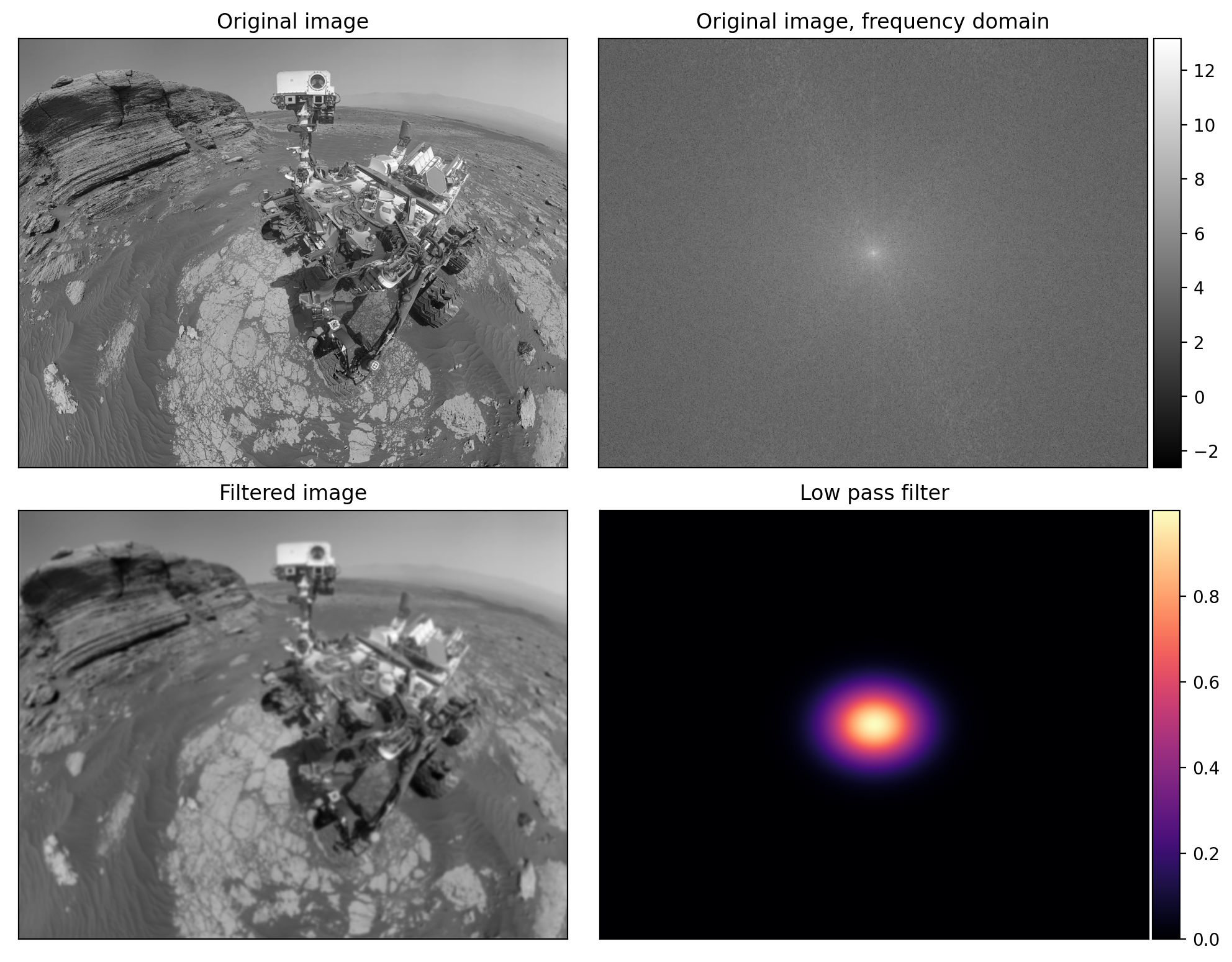
Let's take a look at how the algorithm works in more detail. Figure 4 shows the first part of the pipeline, where we apply a low-pass filter to blur the initial image. The image is first converted into frequency space. There the Gaussian filter is applied by multiplying it with the spectrum (the alternative would be to do a convolution in image-space). After that, the image is reconstructed using the inverse Fourier transform, producing a blurrier and denoised version.

More concretely, we compute the 2D FFT of the initial image, $\tilde{E}(u, v) = \text{FFT}^2\{ E[n, m]\}$. Then the frequencies $u$ and $v$ are converted to polar coordinates, from which we use only the magnitude $r_{i,j} = \sqrt{u_i^2 + v_j^2}$. For the low pass filter, we can use a Gaussian filter, whose functional form in the spatial and frequency domain is

$$ g(x) = \frac{1}{\sqrt{2 \pi} \sigma } e^{\frac{x^2}{2 \sigma^2}} \iff \tilde{g}(f) = e^{-f^2 / (2 \sigma^2)} $$

The filter is evaluated in frequency space for all magnitudes $r_{ij}$, producing a grid of multiplicative factors, shown in the bottom right plot of Figure 4. As we can see, the values are non-zero only for the smallest frequencies (traditionally plotted in the center of the image). This means that by multiplying it with the spectrum we "extinguish" the effect that any high frequencies might have in the image. And as a result, the inverse 2D FFT produces a blurrier and denoised image.

The low-pass filter modifies only the amplitudes of the waves. Next, we have to apply the phase stretching. The frequencies are again converted into polar coordinates and only the magnitude $r_{ij}$ is used. Using the hyperparameters $S$ and $W$, we compute the phase kernel $\phi(r)$ which is shown in the first image of Figure 5. Importantly, the phase kernel has low values close to 0 for the smallest frequencies - those in the center, as is customary to plot spectrum-like 2D grids. The higher frequencies receive a higher phase, up to the limit $S$. The warping parameter $W$ controls how fast the added phase increases radially.

Having computed the phase kernel $\phi(r)$ we multiply $e^{i \phi(r)}$ with the 2D Fourier spectrum of the filtered image, take the inverse 2D FFT, and normalize the result to be in $[0, 1]$. The resulting features are shown in the second image of Figure 5. The transform is now complete and any edges or corners have been enhanced. For the sake of better visualisation, we can binarize the image. Here we compute the 85-th percentile of the feature values and set all pixels with intensity below that value to $0$. Similarly those with intensity values above the threshold are set to $1$. This produces the final black-and-white image.

Our testing image of the Curiosity rover contains a lot of edges and as a result the final image is full of detail. If one wants to obtain only a semantic subset of the edges (e.g. those of the rover, but not of the rocks) tweaking the hyperparameters may not help much if both the desired and undesired edges have similar phase strengths. Nonetheless, with a bit of tuning and visual inspection one can easily achieve good and sharp edges without any added noise or edge tear.

References

[1] Zhou, Y., MacPhee, C., Suthar, M., Jalali, B. PhyCV: The First Physics-inspired Computer Vision Library arXiv preprint arXiv:2301.12531 (2023).
[2] Mahjoubfar, A., Churkin, D., Barland, S. et al. Time Stretch and Its Applications Nature Photon 11, 341–351 (2017).
[3] Asghari, M. H. and Jalali, B. Edge Detection in Digital Images Using Dispersive Phase Stretch Transform. International Journal of Biomedical Imaging (2015).
[4] Asghari, M. H. and Jalali, B. Physics-inspired image edge detection IEEE Global Conference on Signal and Information Processing pp. 293-296 (2014).