Options Pricing
A European call option is a contract that provides its holder the right, but not the obligation, to buy a specific quantity of an underlying asset at a pre-specified strike price on a specified future date. Thus, if you believe that, say, crude oil will increase in price next summer, you can buy a call option from the seller. If the oil price next summer does skyrocket, you can exercise the option and buy the pre-specified amount at the strike price, which is lower than the actual one. If instead, the oil price plummets, you don't have to exercise the option. You'll only lose the price you paid for the option. So, effectively, by buying an option you are buying, literally, an option, an opportunity for a better transaction. Yet, even this opportunity has to have a market price, given that somebody is willing to sell it or buy it. What should it be? How are options priced?
The end-goal here is to derive the famous Black-Scholes model, which is used to infer a theoretical price for European-style options. There will be some math involved, handwavy at times. It all starts with a stochastic process. A stochastic process is a sequence of random variables that can be indexed by some set (e.g. time). There are many examples:
- Discrete time, discrete space. Examples here include the sequence of random variables where at each integer time you move ±1 with equal probability. Alternatively, a Markov chain with a finite number of states. Alternatively, branching processes like Galton–Watson, which counts a population's size at each generation.
- Discrete time, continuous space. Here an example could be the sequence of numbers formed by sampling a stock's price exactly at the end of every hour. Alternatively, autoregressive models like \(AR(1)\), common in time series analysis.
- Continuous time, discrete space. Good examples here include Poisson processes and queuing theory, where objects come at random continuous times, but the number of objects is discrete.
- Continuous time, continuous space. This class includes processes like Ornstein-Uhlenbeck, which is a correlated mean-reverting process (used e.g. in the DDPG model in RL to drive exploration). Similarly, Cox–Ingersoll–Ross is used to model interest rates in economics. But the classic example is the Wiener process which describes the Brownian motion of particles.
Understanding the Wiener Process
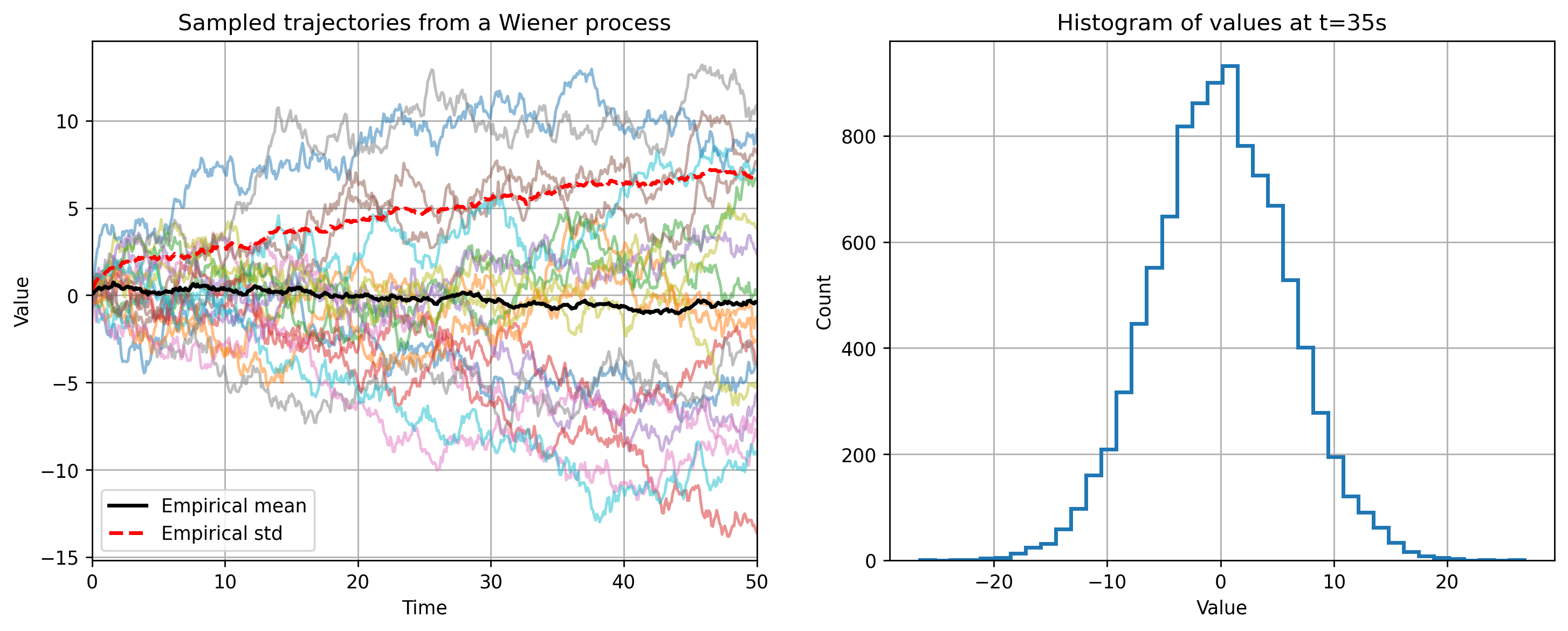
The Wiener process \(W_0, W_1, ...\) is a fundamental stochastic process that pops up in many places, including the Black-Scholes model. It's the unique process with the following properties:
- Starts at zero, i.e. \(W_0 = 0\) almost surely.
- Has independent Gaussian increments. This means that if we pick two timesteps \(s < t\), the process at these steps satisfies \(W_t - W_s \sim N(0, t - s)\). The variable \(W_t - W_s\) is independent of any previous values before \(t\).
- \(W_t\) is almost surely continuous in \(t\).
The variance of the process grows linearly with time. Additionally, the Wiener process is memoryless, or Markov - if \(s\) is the current step and \(W_s\) is its value, the distribution at a later time \(t\) depends on \(W_t\) at \(s\) but not on anything earlier than \(s\). It's also a martingale - the expected value at any future \(t\) is the current value \(W_s\). In other words, if we want to predict any future value, the best prediction in a MSE sense is the current value.
Besides these, another interesting implication from property 2 is that it's nowhere differentiable. To see this, consider that \(W_{t+h} - W_t \sim N(0, h)\). For a typical difference between \(W_{t+h}\) and \(W_t\) one can use the root mean square (RMS), \(\sqrt{\mathbb{E}[W_{t+h} - W_t]^2}\), which is equal to \(\sqrt{h}\). Hence for the finite difference in the derivative we get \(\lim_{h \rightarrow 0} (W_{t+h} - W_t)/h = 1/\sqrt{h} = \infty\). The Wiener process is "too rough", in time \(dt\) the value changes by \(\sqrt{dt}\) and the derivative doesn't exist.
The Wiener process plays a key role in defining other stochastic processes. To see this, consider the cumulative sum of many tiny independent increments. Suppose we take the range \([0, T]\) and cut it into \(N\) boxes, so that \(\Delta t = T/N\). For each box we have an i.i.d random variable \(\Delta X_N\). The variable in box \(k\) is \(\Delta X_{k, N}\). All these variables come from the same distribution and suppose their means and variances are \(\mathbb{E}[\Delta_{k, N}] = \mu \Delta t\) and \(\text{Var}(\Delta X_{k,N}) = \sigma^2 \Delta t\), respectively. Let's further assume the distribution admits no huge outliers (we'll keep this rather informal). Now, the central object of interest is the cumulative sum of these variables up to some \(t \in [0, T]\) and its statistics:
One can see that as \(N\) increases, \(\Delta t\) decreases, and the mean of \(X_N(t)\) converges to \(\mu t\) while the variance to \(\sigma^2 t\). Furthermore, the entire variable \(X_N(t)\) converges in distribution to a Gaussian \(N(\mu t, \sigma^2 t)\). This argument is involved, but is similar to the CLT. Now, if we take the difference between two elements, \(X_N(t + \Delta t) - X_N(t)\), it equals \(\mu \Delta t + \sigma \sqrt{\Delta t}Z\), where \(Z \sim N(0, 1)\). The mean of this difference is \(\mu \Delta t\) and its derivative is \(\mu\), while for the random part its slope is \((\sigma \sqrt{ \Delta t} Z)/\Delta t\) and blows up like \(O(1/\sqrt{\Delta t})\). One can recognize the white noise or the Wiener process from this. If we denote a small change in the Wiener process as \(dW\), we can write:
This is interesting, we started with finite i.i.d increments from any reasonable distribution with no large outliers and we got that as \(\Delta t \rightarrow 0\) the change equals a trend (drift) term linearly increasing in \(dt\), and some white noise, Wiener component. One can intuitively see that any such stochastic process can be formulated as \(dX_t = \mu(X_t, t)dt + \sigma(X_t, t)dW_t\), and this will be the notation we'll use. Тhe \(dX_t\) is to be interpreted not as an actual derivative, but a small change at time \(t\). Therefore, a small change in \(X_t\) is caused by a small drift term and a small addition of noise.
Itô's Lemma
Now that we know what is, roughly, a continuous time continuous space stochastic process, the next step is to understand how to take the derivative of a function \(f\) of that stochastic process. This means that if \(X_t\) is a stochastic process, and \(x\) is a particular realized value at time \(t\), and there is a function of interest \(f(t, x)\), we want to find \(df(t, X_t)\), which shows how the function \(f\) changes.
Suppose \(dX_t = \mu dt + \sigma dW_t\), where \(\mu\) and \(\sigma\) represent the drift and diffusion terms and can depend on \(t\) and \(X_t\). To derive \(df/dt\), we expand \(f(t + \Delta t, X_{t + \Delta t})\) to second order in \(\Delta t\):
Here one should be careful with the notation - \(f_t\) is the derivative of \(f\) with respect to \(t\), not the value of \(f\) at time \(t\). Same for \(f_x\) and \(f_{xx}\). Now, \(\Delta X_t = \mu \Delta t + \sigma \Delta W_t\), and \(\Delta W_t\) grows as \(O(\sqrt{\Delta t})\). So for the \((\Delta W_t)^2\) term we get
In the last line anything that goes to zero faster than \(\Delta t\) is removed. After rearranging, we get
This last formula is called Itô's lemma and represents a cornerstone equation in the field of stochastic calculus. Unlike the classical chain rule, here we pick up a \(\sigma^2/2 \cdot f_{xx} dt\) drift correction term from the process’s quadratic variation. That small extra bit drives everything non-intuitive in stochastic calculus. Even though \(W_t\) has no classical derivative, Ito’s lemma gives us a rigorous “chain rule” for functions of \(W_t\).
Black-Scholes Model
Finally we get to the finance application. First, consider the geometric Brownian motion (GBM) \(dX_t = \mu X_t dt + \sigma X_t dW_t\), with \(X_0 > 0\). We apply Itô's lemma on the function \(Y_t = \ln X_t\), which gives \(dY_t = (\mu - \sigma^2 / 2)dt + \sigma dW_t\) and shows that geometric Brownian motion is just Brownian motion in the log-space. If we want to solve this, we integrate
Consider a simple call option. Suppose the price of the underlying asset, say stock, is \(S_t\) and it is modeled as a geometric Brownian motion process. Further assume there is no arbitrage, markets are frictionless, and there's a constant risk-free rate of return \(r\). The option price for that asset is given by \(V = V(S, t)\). Its derivatives are \(V_t\), \(V_S\) and \(V_{SS}\). Applying Itô's lemma gives us
Now, consider that if a call option is in the money (it's profitable for the holder to exercise it), any increase in the underlying stock's price will increase the profit for the holder and reduce it for the writer (the person who is obligated to fulfill the contract). Since the stock price \(S_t\) fluctuates randomly, the writer is exposed to risk. He can avert a possible loss by owning the underlying stock, so that even though he'll lose more from exercising of the option, he'll gain more from owning the stock. Likewise, if it's not profitable to exercise the option, the writer should not own any of the shares of the stock, otherwise their value will decrease. If \(S_t\) starts going down, the writer can sell any stock units he owns. Thus, we see that the writer can eliminate the underlying risk of the option by owning appropriate quantities of the underlying asset. This is called dynamic hedging.
The writer's hedged portfolio looks like \(\Pi = V - \Delta \cdot S\). He sells the option, so he receives \(V\). He also buys \(\Delta\) units worth of stock at the current stock price \(S\). The question is how to determine \(\Delta\). We'll do this by forming a delta neutral portfolio which trades stocks so that it offsets the changes in the option price. An infinitesimal increase in the option price \(dV\) has to be offset by holding a certain amount of stocks \(\Delta\), whose price changes by \(dS\). Therefore we set it to \(\Delta = V_S = \partial V/ \partial S\). A change in the hedged portfolio is then \(d\Pi = dV - V_S dS\). We already determined \(dV\) above, while \(dS\) is simply a geometric Brownian process \(dS = \mu S dt + \sigma S dW\). By substituting and simplifying the \(dW\) term cancels out and we get
That’s how choosing \(\Delta = V_S\) hedges away all randomness, leaving a purely deterministic growth term. This does assume that the market has no transaction costs, no spread, infinite liquidity and so on. But now that the hedged portfolio has no risk, it must earn the risk-free rate \(r\):
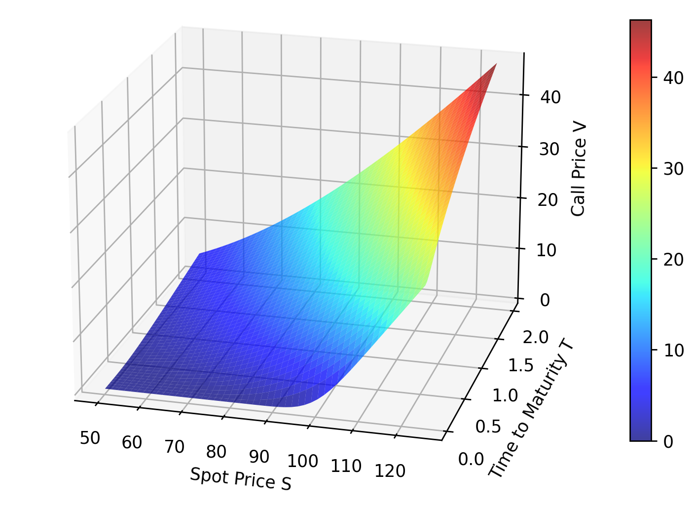
With this last step we reach the Black-Scholes partial differential equation. The equation that spawned multi-trillion dollar industries like exchange traded options, over-the-counter derivative securities, credit default swaps, and securitized debt. After solving it one obtains
where \(V\) is the price of a European call option, \(S\) is the current stock price, \(K\) is the strike price, \(T - t\) is the time to maturity (in years), \(r\) is a continuously-compounded risk-free rate, \(\sigma\) is the stock volatility (annualized std. deviation), and \(N(\cdot)\) is the Gaussian cumulative density function.
Finally, one should recognize that the Black-Scholes equation above does not represent the ground-truth when it comes to real-life realistic modeling. In the real world stock prices don't move according to geometric Brownian motion - there's episodes of increased correlated volatility as well as calmness. Additionally, stock prices often have long tails caused by rare events that bring new information into the market. These in turn lead to jump processes. The resulting integro-differential equations are all around more complicated, with no closed form solution and require numerical methods. It often happens that due to jumps stock prices far away from the current one may affect the option price. Evidently, pricing opportunities is not easy, but it is exciting.