Markov Chain Mixing Times
Markov chain techniques have proven themselves incredibly valuable in fields like statistics and machine learning where the goal is to sample from a distribution whose density is too complicated to calculate analytically. Algorithms like Metropolis-Hastings produce samples from the required distribution by iterating a discrete stochastic process where the next state depends only on the current state (this being the Markov property). The typical statistical treatment of such an algorithm ends somewhere around here - you implement the algorithm, you let it run for a predefined number of steps, and you assess the quality of the results by looking at outputs like trace plots, autocorrelation plots, and burn-in periods. However, like any other algorithm, Markov chain sampling algorithms have a time complexity which can be analyzed... and computer science has a lot to say about that.
The runtime of Markov chains is a beautiful topic which I find very interesting. Most of the content and examples for this post are taken from C. Moore's and S. Mertens' The Nature of Computation which contains an awesome overview of the ideas in this area.
Basics
We begin by recalling some basic facts about Markov chains.
Markov chains are stochastic processes where the probability of the next state in time \(t+1\) depends only on the current state at time \(t\). We'll be mostly interested in discrete Markov chains which can be represented as (possibly infinite) directed graphs where the nodes are the states and the edges are the transitions. The chain is irreducible if any state \(y\) is eventually reachable with non-negative probability from any chain \(x\). If also, for every state \(x\) in which we start, there is a number of steps \(t\), such that for all \(t' \ge t\), the probability of returning to \(x\) is positive, then this chain is aperiodic. If a Markov chain with finitely many states is irreducible and aperiodic, then it is ergodic - it will always converge to a unique equilibrium distribution as \(t \rightarrow \infty\).
The Markov chain can be represented as a stochastic matrix where the value in row \(i\) and column \(j\) shows the probability of moving to state \(i\) if we are currently in state \(j\). If the chain is ergodic, this matrix has an eigenvalue of 1, whose eigenvector is the equilibrium distribution. All other eigenvalues have an absolute norm less than 1.
Typically, we're interested in quantifying how close is the current distribution over the states at time \(t\) compared to the equilibrium distribution. This can be done with the total variation distance:
Consider this example, we have a Markov chain with two states. From state 1 we always transition to state 2, while in state 2 we move to state 1 with 50% probability and remain in state 2 with 50% probability. Then the stochastic matrix corresponding to this Markov chain is \(\small M = \begin{pmatrix} 0 & 1/2 \\ 1 & 1/2 \end{pmatrix}\). Its eigenvalues are \(1\) and \(\lambda = -\frac{1}{2}\), and the corresponding eigenvectors are \( \small P_{eq} = \begin{pmatrix} 1 \\ 2 \end{pmatrix}\) and \(\small v = \begin{pmatrix} 1 \\ -1 \end{pmatrix}\). The eigenvectors form a basis and therefore any distribution over the states at \(t=0\), for example \( \small P_0 = \begin{pmatrix} 1 \\ 0 \end{pmatrix}\), can be represented as a combination of the equilibrium distribution \(P_{eq}\) and the other eigenvector \(v\): \( P_0 = P_{eq} + \frac{2}{3}v\). The distribution after \(t\) steps is then
Importantly, as \(t \rightarrow \infty\), the memory of the initial state decays exponentially fast as \(\|\lambda \|^t = 2^{-t}\) and as a result the total variation decays similarly
The number of steps needed to reach a small distance \(\epsilon\) from \(P_{eq}\) is given by \(t = \log_2 \frac{2}{3\epsilon} = O(\log \epsilon^{-1})\), which motivates the definition of mixing time - a "loose" measure of the runtime, or computational complexity of that Markov chain. The \(\epsilon\)-mixing time is the smallest \(t\) such that irrespective of the starting distribution, at time \(t\) the total variation between \(P_t\) and \(P_{eq}\) is at most \(\epsilon\):
In reality, what we are interested in is how the mixing time depends on \(n\) - the system size, not \(\epsilon\) per se, because this allows us to understand how the mixing time scales with larger and larger problem instances. The total number of possible states \(N\) could be exponentially large in \(n\) (as in Ising models or graph coloring problems) and to be able to sample from such large spaces we'll need polynomial mixing times in \(n\), i.e. \(\tau = O(\text{poly}(n))\). An optimal mixing time which we call rapid mixing is when \(\tau\) scales as \(O(n \log n)\).
Spectral Analysis
From the toy example above we saw that the mixing time is related to how fast the memory from the initial state decays, which is in turn related to the eigenvalues of the stochastic matrix. We can use spectral theory - a mathematical formalization that allows the idea of eigenvalues & eigenvectors to be applied to other more general structures and phenomena - to derive general bounds on the mixing time.
Similar to above, the system size will be \(n\) and the number of possible states will be \(N\). Then, the Markov chain will be defined through a stochastic \(N \times N\) matrix \(M\) expressing the probabilistic dynamics. The equilibrium distribution \(P_{eq}\) is \(v_0 = P_{eq}\) and its corresponding eigenvalue is \(\lambda_0 = 1\). Then, the important quantity is the spectral gap
The spectral gap is just the difference between the two largest eigenvalues by absolute size (the first of which is always \(1\) for any stochastic matrix). In the toy example above we saw that the non-equilibrium part of the probability decayed according to \(\lambda^t\) so intuitively, if the second largest eigenvalue is small, this decays very fast and the chain takes little time to mix. This suggests that a large spectral gap means faster mixing and a small spectral gap means slow mixing.
Why look only at the second largest eigenvalues by absolute size? In reality, it is true that a Markov chain on 50 states will have its state probability determined by 49 non-equilibrium eigenvectors. If we calculate them, we can calculate exactly how much influence each one of them has and compute the mixing time \(\tau_\epsilon\) exactly. However, for practical problems this is unfeasible, given that \(N\) is typically exponential in \(n\). In such cases, what suffices is to use only the second largest eigenvalue to obtain an upper bound on the total-variation distance, and therefore the mixing time. This is still enough to provide at least an estimate for the order of magnitude of the mixing time.
Speaking of bounds on the mixing time, thinking in terms of spectral gap provides the following result.
Theorem: Let \(M\) be an ergodic, symmetric Markov chain, obeying the detail balance condition. Also let \(M\) have \(N\) states and a spectral gap \(\delta\). Then, for sufficiently small \(\epsilon\) the mixing time is bounded by
If we set \(\epsilon\) to some small value, we get \(\frac{1}{\delta} \lesssim \tau \lesssim \frac{\ln N}{\delta}\) or in other words \(\tau = \Omega(\frac{1}{\delta})\) and \(\tau = O(\frac{\ln N}{\delta})\). Note that if the spectral gap is polynomial in \(n\), then the mixing time is polynomial. If the spectral gap is exponential in \(n\), then the mixing time is also exponential, although the above relationship does not show the exact exponent.
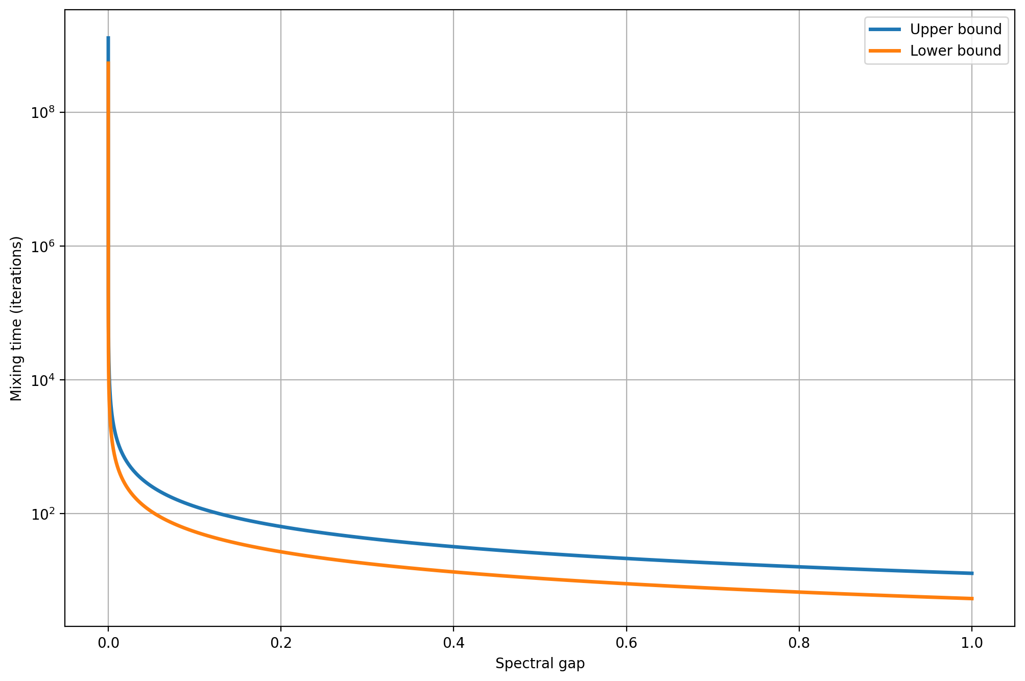
The following plot shows how the mixing time bounds depend on the spectral gap when fixing \(\epsilon=10^{-5}\) and \(N=4\). Since the spectral gap appears in the denominator of the expressions, a chain with a very small spectral gap may require a very large number of iterations to mix well.
We can build some more intuition by running two simple numerical examples. In the first one, we'll measure the tightness of the bounds and the mixing time for a chain with a relatively large spectral gap. In the second example, we'll do the same but for a graph with a very small spectral gap.
For the first example, we have the following well-connected Markov chain.
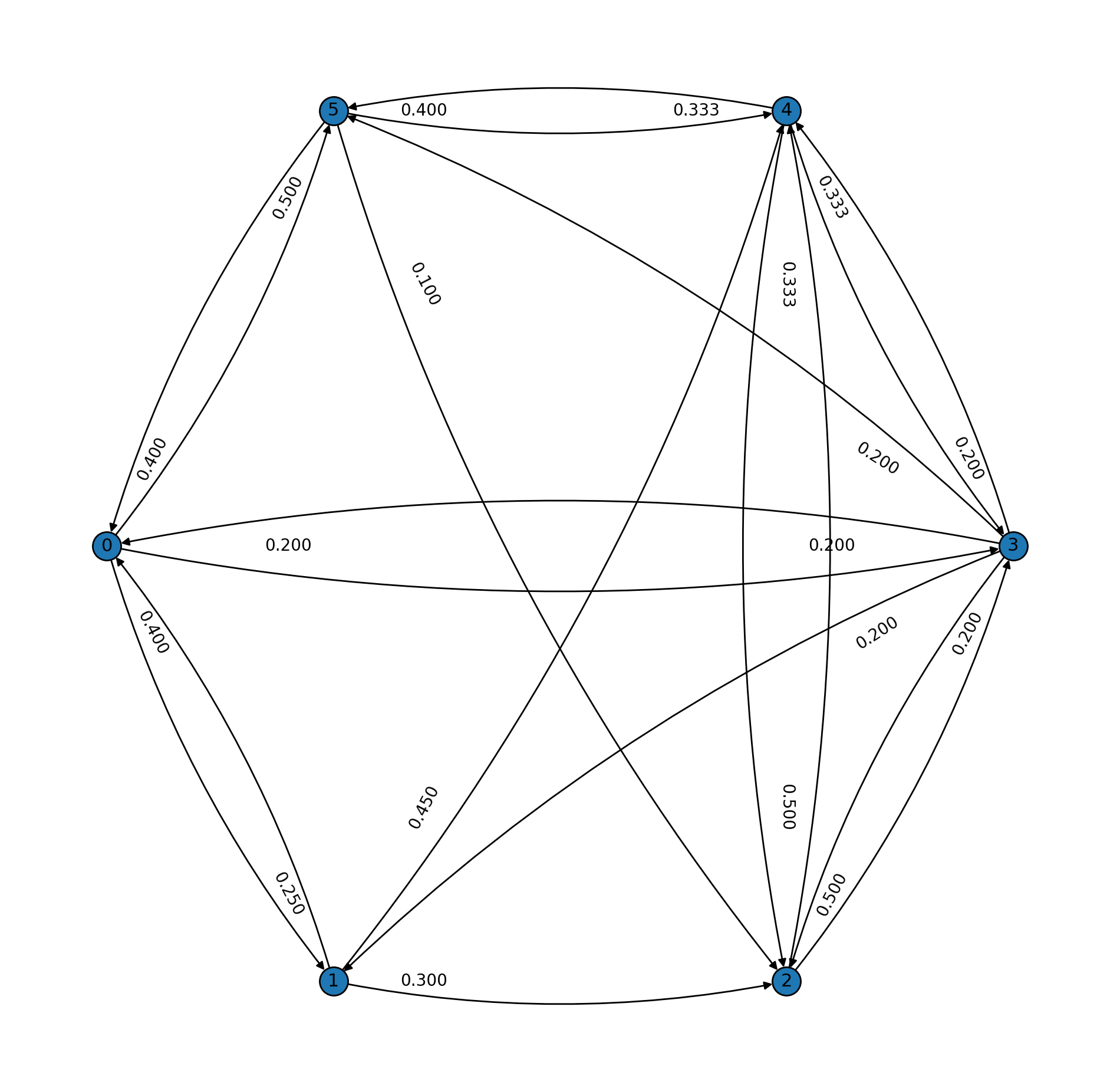
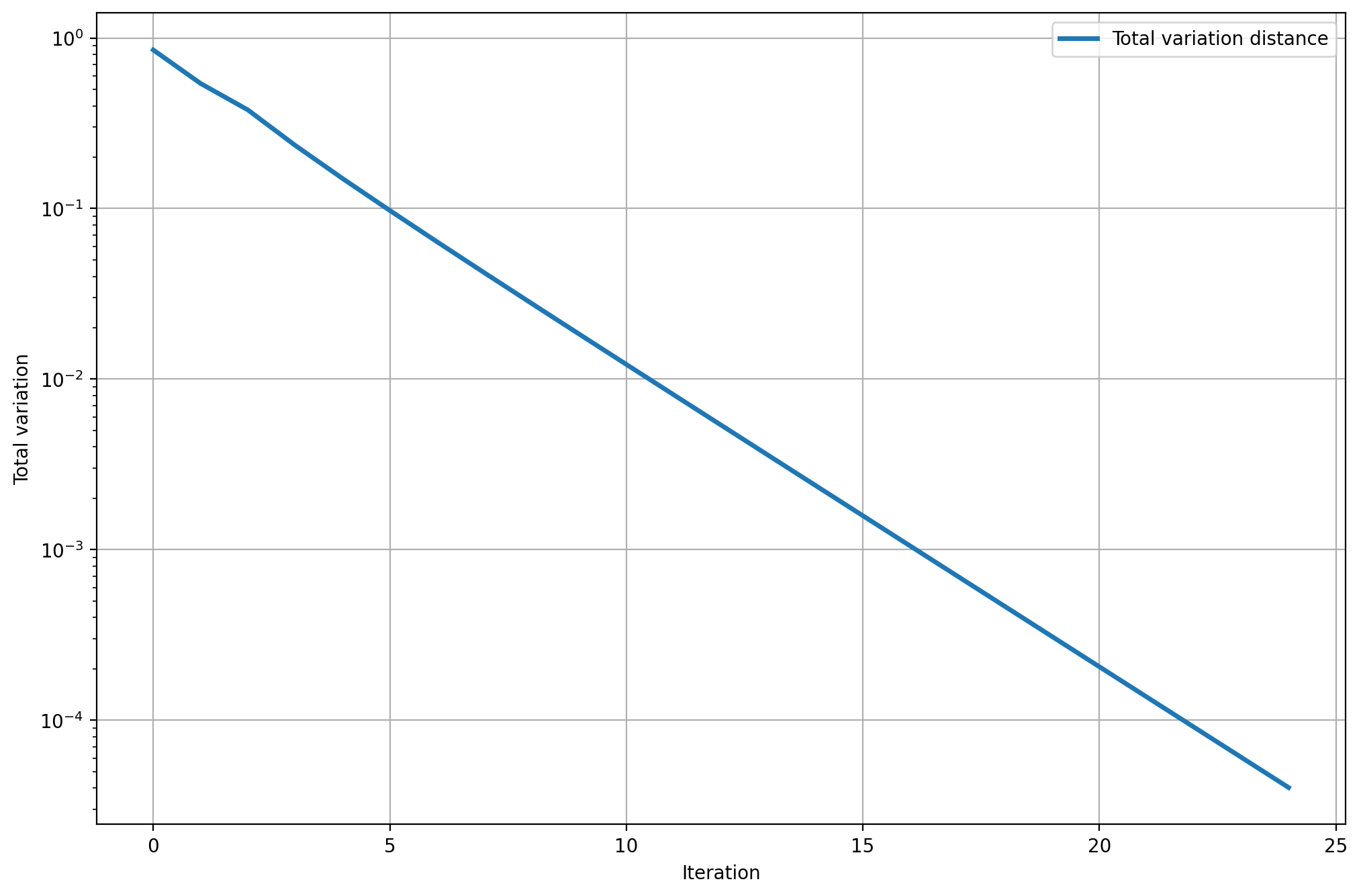
Its spectral gap is approximately \(0.33\), which implies that convergence is relatively fast, compared to the second example we'll see. The following plot shows that if we let the chain run, the state distribution converges exponentially fast toward the equilibrium (note that the \(y\)-axis is logarithmic). It takes only around 23 steps for the total variation to drop below \(10^{-4}\).
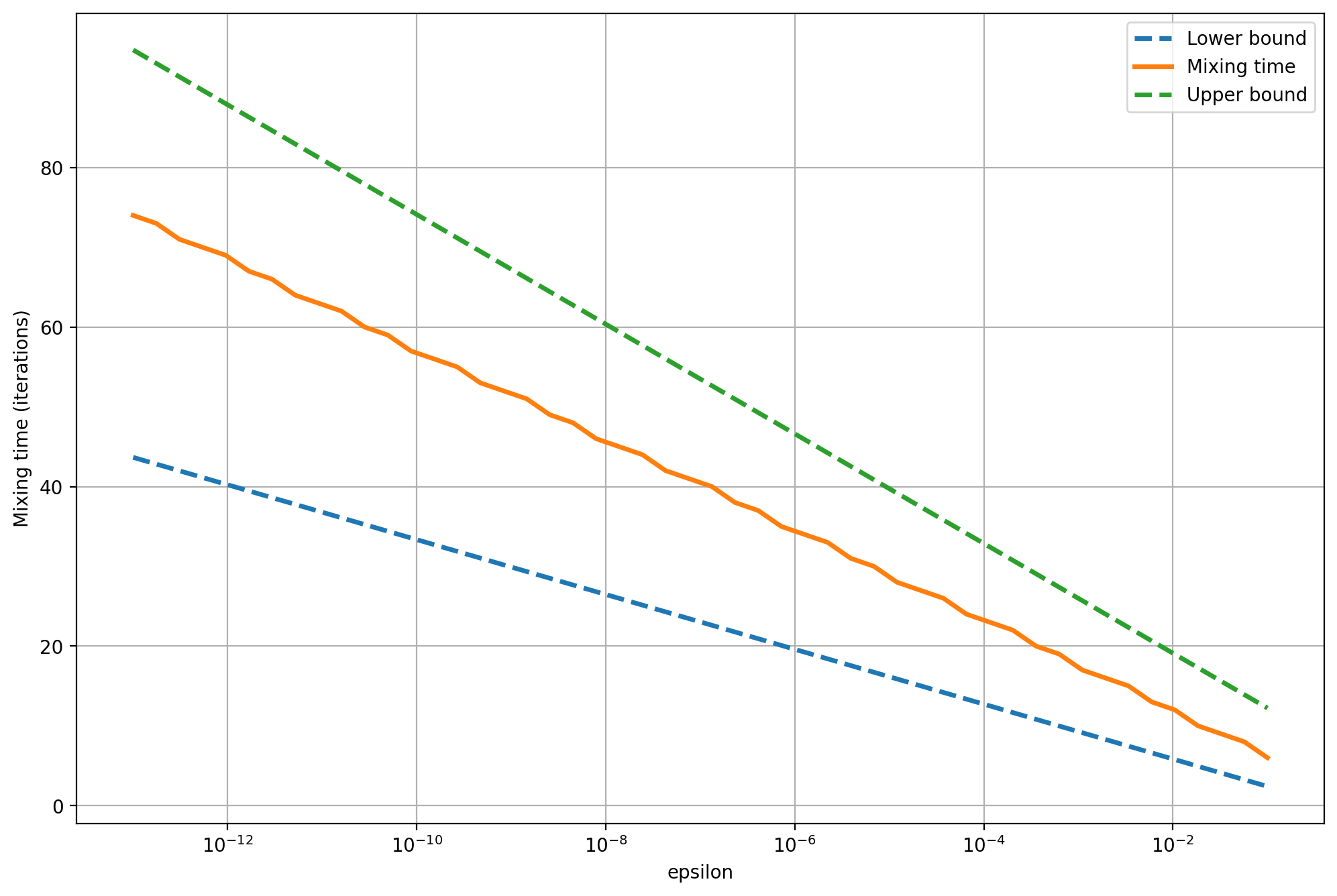
We can also see how tight the bounds are when we vary \(\epsilon\). In the next graph, the \(x\)-axis shows \(\epsilon\) - our total variation tolerance - and the \(y\)-axis shows the mixing time, in iterations, it takes for the total variation to become less than that amount. The results suggest that once the total variation drops below a certain amount, we can make it arbitrarily small by waiting a few more iterations (logarithmic \(x\)-axis). That is one reason why it's more useful to focus on how the mixing time depends on \(n\), not \(\epsilon\). This is not shown on this plot because we keep the graph fixed.
Now, let's take a look at the second example which has, again, few nodes, but with a very small spectral gap. We can think of this graph as having two well-connected components where the transition probabilities inside each component are almost uniform, but the transition probabilities between the two components are almost zero. This creates a natural difficulty in how the random walk can "flow" through the two components.
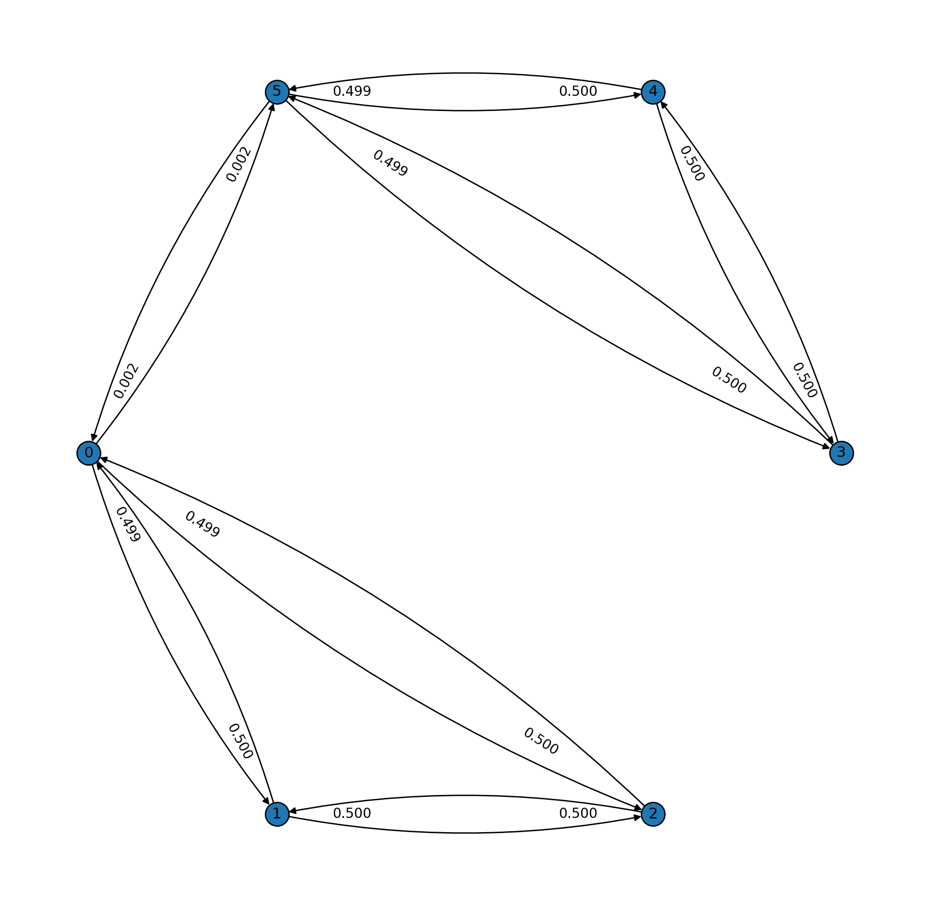
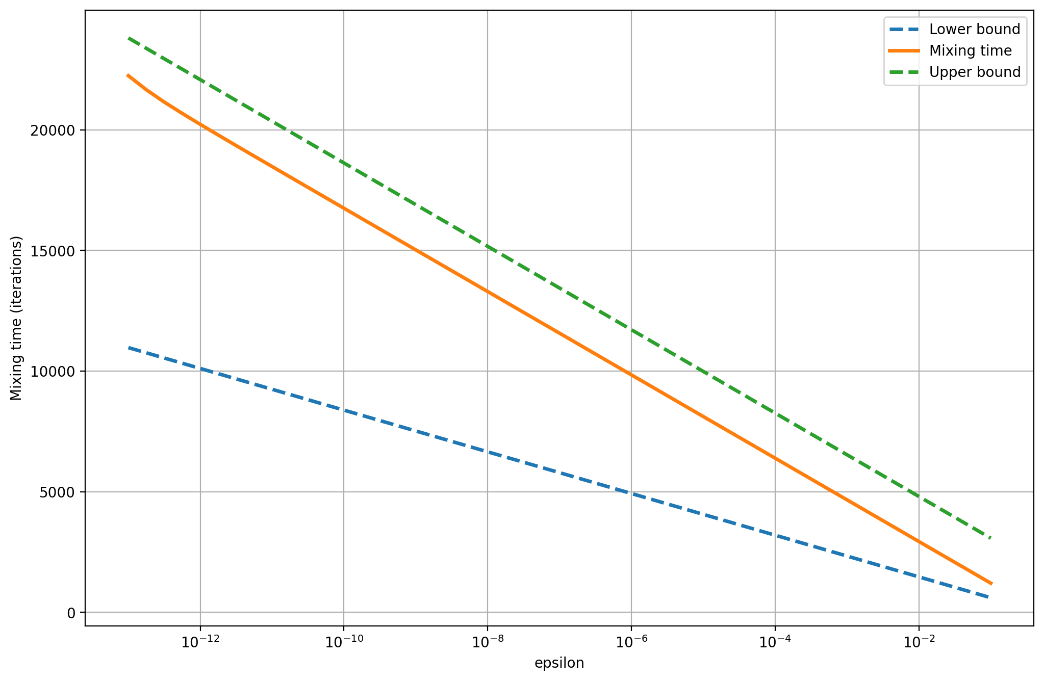
The spectral gap is approximately \(0.001\). The bounds and the actual mixing time are much higher, as the following plot shows. To drop the total variation under \(10^{-10}\) requires about \(20000\) iterations, or about \(285\) times the number needed when the spectral gap is \(0.33\).
Conductance of Probabilities
The last numerical example showed that the mixing time is related to whether the chain has any "bottlenecks" - subsets of nodes for which the probability of the walk moving out of them (or escaping) is low. This flow of probability is very similar to conductance in an electric circuit.
If \(M\) is the Markov chain and \(x\) and \(y\) are two adjacent states, the flow of probability from \(x\) to \(y\) at equilibrium is \(Q(x \rightarrow y) = P_{eq}(x)M(x \rightarrow y)\). The total flow outside of a region of nodes \(S\) is similarly \(Q(S, \bar{S}) = \sum_{x \in S, y \not \in S} Q(x \rightarrow y)\). Therefore, then the probability of escaping \(S\), given that we are in it, is
Finally, if we shorten \(\sum_{x \in S} P_{eq}(x)\) to \(P_{eq}(S)\), the conductance of the Markov chain is the probability of escaping from the most inescapable set \(S\).
The requirement that \(S\) has at most \(1/2\) equilibrium probability is needed because by allowing \(S\) to be very large, the conductance outside of \(S\) naturally goes down, as \(\bar{S}\) has less and less nodes in it.
An important result linking the spectral gap and the conductance is the following.
Theorem: If \(M\) is a ergodic, symmetric Markov chain with nonnegative eigenvalues, then its spectral gap \(\delta\) and conductance \(\Phi\) are related by
Combining this result with the previous one, the mixing time, for fixed \(\epsilon\), is bounded by
With the concept of conductance defined, one practical benefit is that it can be proved that the mixing time of a random walk on any undirected graph is polynomial in the number of nodes. Since the random walk chooses the next node to move to uniformly from the current neighbors, this prevents the existence of any states to which the flow is disproportionately small. While in reality, our purposefully-constructed chains are not random walks, this result is still useful, as it is one of the few places where we can get bounds on the mixing time depending on the problem instance size.
That being said, it is now time to discuss one particularly beautiful object - an expander graph.
An expander is a graph that has no bottlenecks. We say that a \(d\)-regular graph \(G=(V, E)\) with \(N\) vertices is an expander if there is a constant \(\mu\) such that for all subsets \(S \subseteq V\) with less than or equal to half the total number of vertices, \(\frac{\|E(S, \bar{S})\|}{d\|S\|} \ge \mu\). Intuitively, \(G\) is an expander if for every cut \(S\) and \(V \setminus S\), there are a lot of edges going out of \(S\) and into \(V \setminus S\). Importantly, if we make \(S\) larger, then the number of edges is also increased proportionally.
Note that the expansion \(\mu\) is also equal to the conductance of a random walk on that graph. This ensures that the chain is well-connected and as a result Markov chains on expanders mix very fast - something very useful for applications.
In reality, any graph is an expander for some \(\mu\). To be useful to solve problems of varying sizes however, we would like to have a family of graphs \(\{G_N\}\) - one or more graphs for every possible number of nodes \(N\) - such that the expansion \(\mu\) is constant as \(N\) increases. If this were not the case, we could imagine a scenario where for some problem of size \(25\), we use an expander with expansion \(3\), but for a problem instance of size \(26\), we have access to a graph with expansion \(1\). This just overcomplicates things, which is one reason we want constant expansion as \(N\) increases. If such an infinite family \(\{G_N\}\) of \(d\)-regular graphs exist, then the following are equivalent:
- For some \(\mu > 0\), \(G_N\) is an expander with expansion at least \(\mu\);
- For some \(\Phi > 0\), the lazy walk on \(G_N\) with a modified transition probability \(M' = (M + I)/2\), has conductance at least \(\Phi\);
- For some \(\delta > 0\), the lazy walk on \(G_N\) has a spectral gap at least \(\delta\).
It turns out, such families of graphs are very common and can be generated using random algorithms. Most random \(d\)-regular graphs are expanders. Few deterministic algorithms for generating expanders exist as of today (see Cayley graphs and the Zig Zag product).
Ultimately, expanders are very useful objects. They can be used to reduce the number of random bits needed to run certain algorithms and are useful constructs in some important proofs. There are many interesting aspects worthy of discussion, which unfortunately become too technical for a quick overview. Therefore, I'll leave them for a future post, for when the muse calls.
