Marching Cubes and Co
The field of computer graphics contains some very nice and insightful algorithms. I wish I had explored them earlier, but it's still not that late. This post describes marching cubes - a ultra-simple algorithm for the extraction of a triangular mesh from a 3D field. This algorithm is widely applicable in all kinds of graphics applications, whether it is volumetric rendering of CT scans in healthcare, or tunnel/cave mapping in an industrial setting. It also combines well with the growingly-popular deep learning NeRF models. There it can be used to render a mesh from the 3D reconstruction.
Marching cubes is not the only clever algorithm worth knowing. We'll start with some basic 3D structures and then move to the volumetric stuff, where marching cube reigns.
Consider point clouds as a relatively simple 3D data structure. A point cloud can be represented as a matrix of shape \((N, 3)\) - \(N\) 3-dimensional points, each representing particular \((x, y, z)\) location. Just by looking at these numbers we can get a pretty good sense of the geometry of the scene, especially if the number of points is sufficiently large. Apart from the location, we can also have additional per-point parameters, like color, opacity, or a normal vector. These are stored into specialized file formats such as .pcd or .ply.
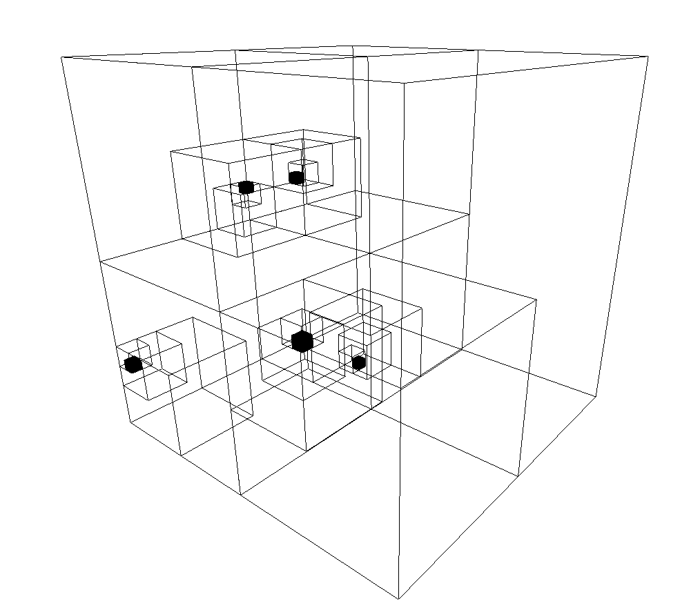
Representing a bunch of points simply as a big matrix is a terrible idea for most purposes. We need specialized data structures, and the octree and \(k\)-d trees come to the rescue. An octree is a tree in which every internal node has up to eight children. It is used to partition the space into 8 octants for easier searching. To build an octree we start with a single giant voxel covering all points. We then split it into 8 non-overlapping octants. Now, we keep subdiving those octants which have more than one point within them, until they have zero or one inside. The larger octants are not subdivided. In such a way a big tree is populated, whose internal nodes can have at most eight children. To insert a new point we start from the root node and progressively navigate down the branches until we find its new place. Searching is handled similarly.
Octrees are the 3D variant of quadtrees. A quadtree divides 2D space into quadrants and subquadrants, representing the points as leaf nodes in a tree whose internal nodes can have at most four children. For both quadtrees and octrees the insertion and deletion of a single element have complexities \(O(\log n)\) where \(n\) is the number of nodes.
K-D trees are similar data structures but with some differences. A \(k\)-d tree is a binary tree and each internal node can have at most two children. At every internal node the points are split according to one coordinate axis - \(x\), \(y\), or \(z\), much like in a decision tree. To create one of these trees we start with the points, choose one axis, e.g. \(x\), and split at the median \(x\)-coordinate of the points we have to insert. Half the points will be to the left of this node, and half to the right. We call the constructor recursively to further split each half until a desired number of points, perhaps one, falls within each subdivision. Search, insertion and deletion are all \(O(\log n)\).
One particular strenght of both the octree and the \(k\)-d tree is the ability to find nearest neighbors efficiently. To find the nearest neighbor of a query point \(p\), we follow the branches according to \(p\)'s location until we reach a leaf node. Its distance to \(p\) is the current minimal distance. Then, we start backtracking up the tree. At each of the internal nodes we compare the distance between \(p\) and the splitting value. If it is larger than the current minimal distance, there's no point in searching the corresponding branch. If it is smaller, then there may be a leaf node that is closer than our current estimate, in which case we have to search that branch. The search ends once we reach the root.

Being able to efficiently calculate closest points allows us to calculate the Chamfer distance between two point clouds. It is given by the symmetric average distance between a point from the first cloud and its nearest neighbor in the other one. It is a fundamental metric used when registering or generating point clouds. It has wide applications for example in autonomous vehicles where generative models predict future Lidar clouds conditional on vehicle motion.
What else can we do with point clouds? There are various options. One can:
- Downsample the points by bucketing them into regularly-placed voxels and averaging all points within each voxel. This has the effect of filtering out noisy points.
- Estimate vertex normals by looking at the neighborhood of each point and computing a principal axis based on the covariance of the points in that neighborhood.
- Crop the point cloud, calculate a bounding box or a convex hull around it.
- Cluster the points into semantically meaningful groups or do plane segmentation to find a 3D plane with maximal number of points lying on it. This is commonly done with RANSAC - that famous absurdly simple, absurdly robust line-fitting algorithm.
Now consider triangle meshes. They consist of \(N\) three-dimensional vertices, perhaps stored in an array of shape \((N, 3)\), and \(M\) faces, which connect the vertices into cohesive surfaces. The faces can be stored in a matrix of shape \((M, 3)\) where the \(i\)-th row contains the indices for the three vertices defining the \(i\)-th face. What can we do with such a mesh? We can:
- Crop, paint, or visualize it. In practice, visualisation looks nicely only with shading enabled, which requires surface normals in order to calculate how much light falls on each surface region, based on its orientation with respect to the light source.
- Filter the surface "roughness" by averaging the vertices in a neighborhood, as given by the connectivity of the mesh. This can make surfaces smoother, but some filters based on this principle, like the Laplacian, can have the problem of thinning the surface too much.
- Sample a point cloud from the mesh. Simple methods like uniform sampling from the vertices may result in some points being clustered. To address this, other methods like Poisson disk sampling can be used.
- Do mesh simplification. This means reducing the number of vertices and faces while keeping the mesh detail quality as high as possible. A simple method here could be just to average the vertices falling in a given voxel.
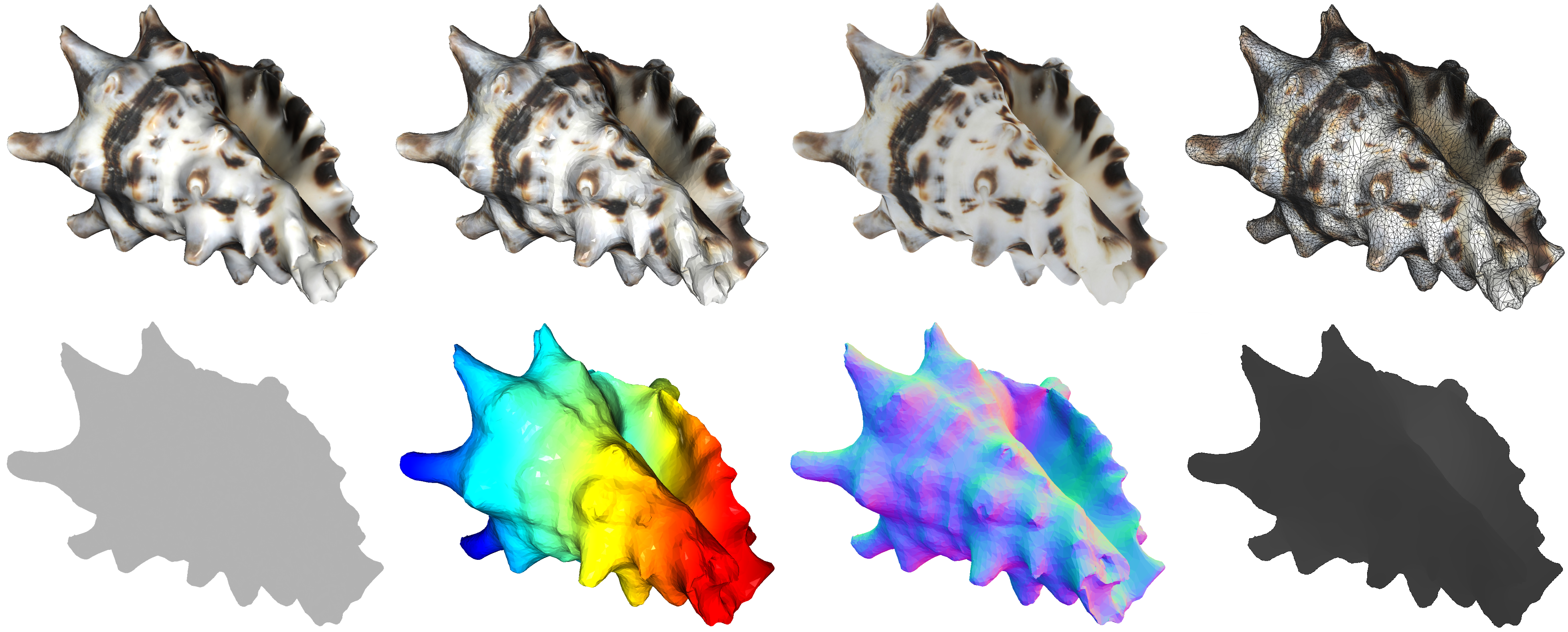
Figure 2 visualizes various characteristics of the mesh like depth, normals, and different shading settings. Note that a triangle face normal is useful in telling us how the face is oriented in 3D. If the shading uses face normals, then it can either apply a constant shade to the whole face - flat shading, or it can evaluate the colors in two neighboring face centers or vertices and interpolate colours/shades in between - Gouraud shading. The former produces discontinuous colors along continuous viewed surfaces, while the latter may produce unrealistic visual artefacts. A slightly more expensive solution is the Phong shading where instead of interpolating colours we interpolate vertex normals. This produces excellent visual results. A separate topic is whether one uses specular reflection in the lightning. The combination of using both a diffuse and specular reflection is called the Phong reflection model.

Going from mesh to point cloud is easy - one can just take the vertices or sample from them. It is more interesting how to go from point cloud to mesh and for this task there is a classic algorithm - ball pivoting. Consider a spherical ball of radius \(r\) which is dropped somewhere on top of the point cloud. If \(r\) is sufficiently large, the ball will hit exactly three points. These points form a triangle from which we will iteratively grow the surface mesh. In this initialization step of the algorithm we just need to find a seed triangle - three points laying on the surface of a sphere with radius \(r\) such that no other points are within the sphere.
Now, we start pivoting the ball across the edges of the triangle. If vertices \(v_1\) and \(v_2\) are joined by edge \(e_1\), we can imagine pushing the ball across \(e_1\), until it lands on a new point \(v_3\), in which case we construct edges \(e_2 = (v_1, v_3)\) and \(e_3 = (v_2, v_3)\), thereby obtaining a new triangle. This process then continues, considering the newly added edges and adding additional triangles. When there are no more points to add, we can choose a different seed triangle and start from it.
Note how the quality of the constructed mesh depends on the radius \(r\). If \(r\) is too large, then you will certainly grow the mesh, but you may miss out on certain smaller non-convex regions and hence the result will be less detailed. If \(r\) is too small, then the ball will "fall" through the point cloud and you will fail to grow the mesh and may end up with multiple meshes forming separate connected components. For that reason, care should be taken in how \(r\) is chosen. Similarly, we also need to check surface normals to assess whether new polygon faces have their orientation aligned with the ones we already have. Additionally, with noisy points the algorithm may create small spurious surfaces that need to be removed in a postprocessing step.
Having an explicit mesh allows us to obtain implicit representations of the object. One popular implicit representation is the signed distance function (SDF) which for every 3D point \(\textbf{x}\) returns a scalar \(y\) which represents the distance to the closest point on the object. If \(y\) is positive, then \(\textbf{x}\) lies outside of the object boundary (which itself is assumed to be watertight, so that the object has meaningful internal/external regions), otherwise it is inside it. If \(\textbf{x}\) is exactly on the object surface, then \(y\) is \(0\).
By being able to find the closest point on a given surface, we can compute the signed distance function for many regularly-placed query points in a 3D grid. The result will be a big tensor with 3 axes, containing dense volumetric data implicitly representing the 3D scene.
Note that volumetric data is where we start getting into NeRF territory. To render a pixel from volumetric data, one needs to shoot out a ray from the camera center through the pixel of interest and integrate the colour/shades of the 3D points along the ray, according to their corresponding densities. Unlike surface rendering, which only represents the outer surface of objects, volumetric rendering represents both the surface and the interior of 3D models. This technique is particularly useful for displaying objects that are semitransparent or have varying properties throughout their volume, such as clouds, smoke, fire, or the human body in medical imaging.
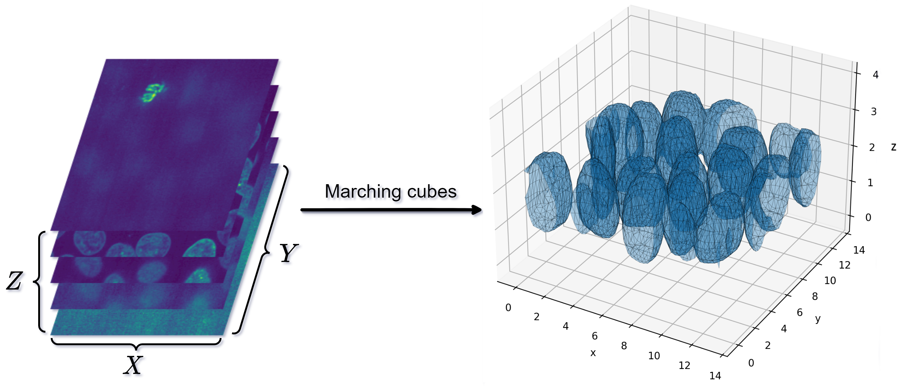
So, suppose we have a volumetric dataset of shape \((X, Y, Z)\) and each entry corresponds to some material density of interest. Medical imaging like CT and MRI scans can produce multiple 2D slices which when stacked result in such a dataset. Similarly, a NeRF model can be evaluated in many points \((x, y, z)\) to produce a learned density field. Once we have the data, we want to find isosurfaces - surfaces whose points have the same value in the volume. The exact value, call it \(\bar{v}\) here is user-selected but for any SDF it makes sense to use set \(\bar{v} = 0\), as we want to find the exact object surfaces.
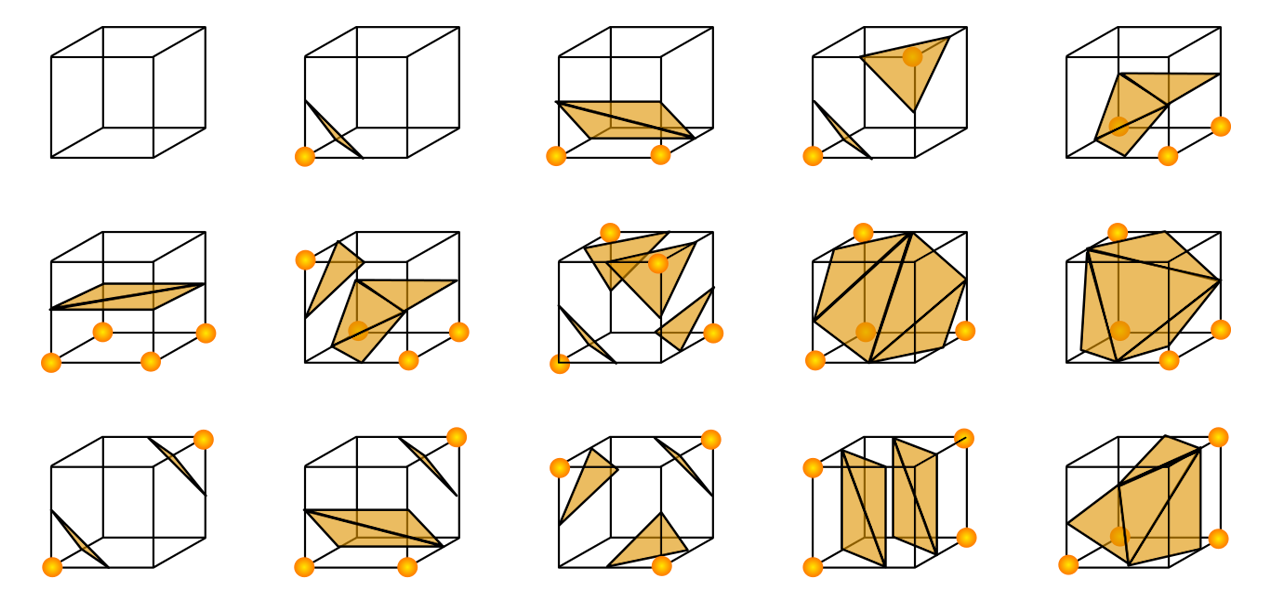
Our datapoints live in a regular 3D grid and we can ennumerate all the grid voxels. Marching cubes, a cornerstone algorithm, works in this manner - it iterates over all voxels and builds triangles from each one independently. Consider one particular voxel. It has 8 vertices at which we have a value. And each value can be above or below our value threshold. If both vertices along an edge have values greater or lower than \(\bar{v}\), then the surface does not cross this edge - we may be inside or outside of the object but the object boundary does not cross that edge. Since the voxel has 8 vertices and each can be below \(\bar{v}\) or otherwise, there are \(2^8 = 256\) different configurations. These can be ennumerated and stored in a table for easy future lookup. Each configuration corresponds to a small set of triangles aligned with the corresponding points. Some cases are shown in Figure 3.

So, marching cubes proceeds by iterating over the grids and creating triangles according to where the values of the vertices are above or below the threshold \(\bar{v}\). This usually results in high-quality meshes, at least as long as \(\bar{v}\) is set properly. Otherwise various floater surfaces may show up or the resulting meshes may not be watertight - something which is required for 3D printing or other downstream applications.
