IS-LM-UIP: Dynamics and Intuition | The Critical Section

This is yet another post on the IS-LM model in macroeconomics, with the twist that this time it's an open economy and I've actually coded it up into a nice dashboard. Needless to say, even though the IS-LM has abysmal predictive power, it captures essential relationships in macroeconomic theory and is a useful educational tool to understand the different market processes. Through a graphical approach, we'll summarize famous economic scenarios and concepts, and we'll explore the role that expectations play within the dynamics.

Model Description

The model in question is simple, but comprehensive. Consumption $C$ is linear in the disposable income $Y - T$. Taxes are $T$ and income, equal to output, is $Y$. Investment is decreasing in the real interest rate $r$. Government spending $G$ is exogenous. Net exports are linear, increasing in foreign income $Y^\ast$, and decreasing in domestic income $Y$ and the real exchange rate $\epsilon$. The central bank sets the money supply $M$ and the LM relation is linear in income and nominal interest rate. We ignore the zero lower bound. The country has perfect capital mobility and therefore the uncovered interest rate (UIP) holds. The exchange rate is floating, so that given the domestic and foreign interest rates $i$ and $i^\ast$, the nominal exchange rate adjusts almost instantaneously.

$$ \begin{cases} Y = C + I + G + NX & \leftarrow\text{IS relation} \\ C = C_0 + C_1(Y - T) & \leftarrow\text{Consumption, linear in disposable income} \\ I = I_0 - I_1r & \leftarrow\text{Investment, linear in real interest rate} \\ r = i - \pi^e & \leftarrow\text{Approximate Fisher equation} \\ \pi^e = \frac{P^e - P}{P} & \leftarrow\text{Expected inflation} \\ NX = n_0 + n_1 Y^\ast - n_2 Y - n_3 \epsilon & \leftarrow\text{Net exports}\\ \epsilon = EP/P^\ast & \leftarrow\text{Real exchange rate}\\ M/P = \phi_0 + \phi_1 Y - \phi_2 i & \leftarrow\text{LM relation}\\ E = E^e \frac{1+i}{1+i^*} & \leftarrow\text{Uncovered interest parity}\\ P = P^e + \alpha (Y - \bar{Y}) & \leftarrow\text{Short run aggregate supply}\\ Y = \bar{Y} & \leftarrow\text{Long run aggregate supply}\\ \end{cases} $$

All coefficients $C_0, C_1, I_0, I_1, n_0, n_1, n_2, n_3, \phi_0, \phi_1, \phi_2, \alpha$ are assumed positive. In particular, $n_3 > 0$ ensures that when the real exchange rate falls, exports increase and net exports improve. This is related to the Marshall-Lerner condition. By assuming linear net exports we avoid the more complicated and ambiguous non-linear equation $NX = X(\underset{+}{Y*}, \underset{-}{\epsilon}) - IM(\underset{+}{Y}, \underset{+}{\epsilon})/\epsilon$. In that equation the imports, paid in the foreign currency, have to be converted to the local one, and this can create nonlinear terms. Finally, the exchange rate is defined as the price of domestic currency in terms of foreign currency. That is, $E = F/D$, with domestic in the denominator. An increase in $E$ is a nominal appreciation. The equations of the UIP and the real exchange rate $\epsilon$ are adjusted accordingly. Variables with a $e$ superscript, like $\pi^e$, are future expectations. The asterisk $^\ast$ indicates foreign quantities of interest.

Let's ignore the last two equations for now. If we substitute everything else, except these two, within the IS-LM we'll get two equations in three variables, $(Y, i, P)$. All other variables can be derived from these. Now, to find a unique solution of $(Y, i, P)$ we need more assumptions. There are two competing assumptions, from which the distinction between short-run and long-run arises. In the short-run the IS-LM assumes that prices are fixed, $P=\bar{P}$. Intuitively, if the prices are fixed, then the IS-LM describes the short-run equilibrium. In the long-run, the classical view is that output is at potential, $Y = \bar{Y}$.

In reality though, prices are not fixed. They're sticky. That's where the short-run aggregate supply (SRAS) comes in. It has a positive slope $\alpha$. On the other hand, we can obtain the aggregate demand (AD) by solving the IS-LM for any fixed price $P$. AD is simply the relationship between the equilibrium IS-LM output and price. With AS and AD determined the short run general equilibrium is at their intersection. The long-run (LR) equilibrium is at the intersection of AD and $Y = \bar{Y}$.

The model described above is linear and can be solved in closed form. The AD can be easily calculated in a vectorized manner across an array of different prices. Intersections of AD and SRAS or LRAS can be found analytically.

Dynamics

Even though there are no actual dynamics within the equations themselves, we can describe them qualitatively and show them by iteratively changing the current values of the model's variables.

Short run transitions. Suppose the executive government (finance ministry) proposes a spending increase and Parliament approves it. As a result, $G$ increases. Suppose also prices are fixed and the central bank keeps the money supply $M$ fixed as well. The sequence of events is as follows:

$$ G\uparrow \ \Rightarrow \ Y\uparrow \ \Rightarrow \ C \uparrow, NX \downarrow, i\uparrow \ \Rightarrow \ Y\uparrow_C, Y\downarrow_{NX}, I \downarrow_r, E\uparrow_{i} \ \Rightarrow \dots $$

Here the notation $Y\uparrow_C$ indicates that $Y$ increases because of $C$. The initial shock increase in $G$ causes an increase in $Y$, which causes changes in the other variables across the economy, which in turn affect $Y$ again, through feedback. The model's design guarantees mathematically that this feedback gradually fades out and the economy, governed by the corresponding amplification mechanism, converges to a new SR equilibrium.

As another example, consider a major improvement in the production process of most firms. As a result the supply-side capacity of the economy increases and $\bar{Y}$ increases. Assuming we start from $Y=\bar{Y}$ and $P=P^e$, here's what follows:

$$ \bar{Y}\uparrow \ \Rightarrow \ P \downarrow \ \Rightarrow Y \uparrow, i \downarrow, \pi^e \uparrow, \epsilon \downarrow \ \Rightarrow \ C\uparrow_{Y}, NX\downarrow_{Y}, P\uparrow_{Y}, E\downarrow_i, NX\uparrow_{\epsilon}, \dots $$

The increase $\bar{Y}$ causes a general price decrease, which among other things, boosts AD and reduces the real exchange rate. These in turn boost consumption, lower net exports through $Y$ but boost it through a lower $\epsilon$ and so on. Tracing the effects quickly becomes overwhelming.

Long run transitions. How does the economy move from short-run to long-run equilibrium? The consensus is that it happens through adjustments of the price expectations $P^e = \mathbb{E}[P_{t+1}]$. The simplest adjustment that converges to the LR equilibrium happens with adaptive expectations, by setting $P^e = P$ at every time period and iterating. If we start above potential output, the economy is overheated. Adaptive expectations then trigger a further price increase which reduces output back to potential value $\bar{Y}$:

$$ P^e \uparrow \ \Rightarrow P \uparrow, \pi^e \uparrow \ \Rightarrow I \uparrow_{r}, \epsilon \uparrow_P, Y \downarrow_P, i \uparrow_P, \pi^e \downarrow_{P}, \dots $$

Note that in this situation consumers only ever see increasing prices and wages. The economy still grows in nominal terms. Yet, in real terms there is a general impoverishment, as due to the rising prices, people can afford less in terms of real goods.

We can simulate the convergence to long-run equilibrium by repeatedly setting $P^e$ to the current $P_t$, recompute the AD-SRAS to obtain new $(Y_{t+1}, i_{t+1}, P_{t+1})$, setting $P^e = P_{t+1}$, recomputing AD-SRAS, setting $P^e = P_{t+2}$ and so on. This process is guaranteed to asymptotically reach $\bar{Y}$. The increased price and a higher interest rate remain permanently.

Adaptive exchange rate expectations. What happens if, in addition to adaptive price expectations, we have adaptive exchange rate expectations, i.e. we set $E^e = \mathbb{E}[E_{t+1}] = E_t$ at every iteration, deviating from standard assumptions? Well, here it gets interesting. If we start above potential output, under adaptive exchange rate expectations we still end up at $\bar{Y}$, with the same consumption $C$. However, $P$, $I$, $NX$, and $\epsilon$ are different compared to their values when exchange rate expectations are fixed. At the fixed point, the UIP says that $E_t = E_t (1+i)/(1+i^\ast)$, from which it follows that the domestic interest $i$ has to be equal to the foreign one $i^\ast$.

Once we acknowledge that with adaptive exchange rate expectations $i = i^\ast$ and $Y=\bar{Y}$, we see that in the LM relation it is the price that has to adjust to accommodate the equality. In a contraction we need $(Y, i)$ to decrease toward $(\bar{Y}, i^\ast)$ and this requires a general price decrease. At the same time $E$ and $\epsilon$ increase rapidly, which hurts net exports. The whole transition is rather complicated but the end result is $Y = \bar{Y}, i = i^\ast$, $P$ is low, and $\epsilon$ is high. For the domestic country, it feels like recession: falling prices, falling real income, and uncompetitive exports.

Fig. 1. An example where the ADAS dynamics under fixed and adaptive exchange rate expectations are completely different. We start from an economy above potential output due to an initial fiscal expansion. Investments are crowded out, $P=3.26, i=12.14, \bar{Y}=300, i^\ast=1, P^*=1$. The domestic currency appreciates and domestic goods become uncompetitive relative to foreign ones. Adaptive exchange expectations makes the path toward long-run equilibrium overshoot potential output $\bar{Y}$ and stabilize from there. Note: results are only qualitative. Model is not calibrated to any real scenario.

Scenarios

Now, let's explore some basic scenarios which can be explained through the IS-LM-UIP.

Paradox of thrift. An increase in the savings rate $1 - C_1$ results in reduced aggregate demand, which in turn reduces income $Y$, which paradoxically results in less savings. In reality, when prices adjust the savings rate will cause increased growth.
Fiscal expansion, crowding out. If $G$ increases, this boosts output in the short-run. However, it increases the interest rate $i$ and reduces investments $I$. Crowding out means that government spending reduces private-sector spending, usually investment.
Fiscal expansion under floating exchange rate. An increase in $G$ triggers, through increased interest rate, a capital inflow and a currency appreciation, which hurts net exports.
Fixed exchange rate defense. If the central bank decides to keep $E$ fixed, then it has to adjust $M$ so that $i = i^\ast$. The LM curve shifts endogenously.
Currency crisis. Expectations of devaluations of $E^e\downarrow$ would immediately cause $E$ to decrease. If the CB has promised to keep $E$ fixed (or within a certain range) it must be ready to buy domestic and sell foreign currency, potentially depleting its reserves.

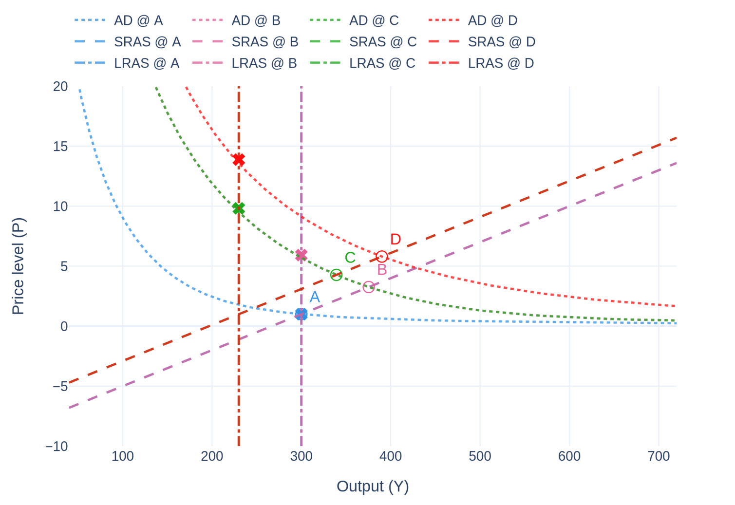
As a final example consider the following story, shown in Fig. 1. We start from long-run equilibrium, point $A$, and the government decides to increase $G$. This brings the economy to point $B$, where output is higher in the short-run, unemployment is smaller than its natural rate, and prices are higher. Suppose a war erupts between two foreign countries soon after. One of them, a major oil producer, restricts its oil exports. As a result, for our domestic firms it becomes more expensive to produce and potential output $\bar{Y}$ drops significantly. The economy transitions to point $C$. To delay the impending crash in $Y$, the domestic central bank decides to increase the money supply, boosting the economy, which now transitions to point $D$. To summarize:

$A \rightarrow B$: fiscal expansion, demand-pull price increase;
$B \rightarrow C$: shock in production process, supply-push price increase;
$C \rightarrow D$: monetary expansion, demand-pull price increase;
After $D$, the economy eventually converges to the red cross, its long-run equilibrium.