Image Histogram Equaliazation
A neat little image processing technique called histogram equalization comes in very handy when one wants to improve the contrast of images. Such a technique may be necessary when an image is either over- or underexposed in which case it would appear too bright or too dark respectively. Likewise, if the distribution of the pixel intensities is sharply peaked around a single value, then any details in the image will be hard to see. In those cases, in order to improve contrast, one simple processing technique is to map the intensity of the colors using a monotonous increasing function to the whole output range. What forms can the function take? Let's find out.
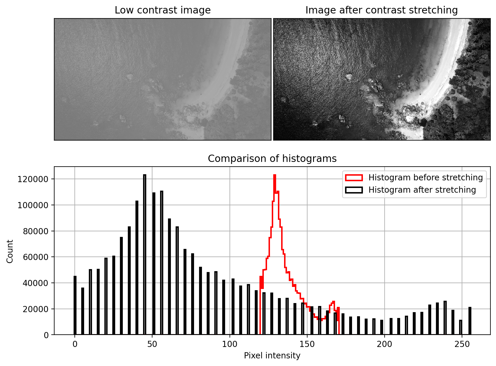
Suppose we have a greyscale image with lots of details in it - object contours, edges, corners, textures - but very low contrast, so that these details are hard to see. The simplest idea of improving contrast is to stretch the intensity values into the full range supported by the image, which would be \([0, 255]\). This is called contrast stretching or sometimes simply contrast normalization and it's a linear transformation applied on the image.
If the initial image has maximum and minimum intensities \(I_{\text{max}}\) and \(I_{\text{min}}\) respectively, the first step is to scale the intensities into \([0, 1]\) using \(\hat{x} = (x - I_{\text{min}})/(I_{\text{max}} - I_{\text{min}} )\). Then we just have to scale it to the desired output range, usually \([0, 255]\), using the formula $\hat{x} = x (O_{\text{max}} - O_{\text{min}}) + O_{\text{min}} $. The final formula is given by:
This applies a linear transformation to the pixel intensities. If the input intensities have a small range compared to the output range, then the transformation will amplify the contrast even between almost similar pixels. As a result, edges are typically amplified making them more easy to see. The downside is that we are changing the intensity balance of the image, which might be undesirable in some situations. For example, if we are taking periodic images of a chemical substance and the colour changes only very slightly, then changing the contrast would not correspond to the real colour of the object captured in the image.
This raises an important point that contrast adjustment techniques should be used only when the reduced contrast is caused by camera-related technical inadequacies. If, for one reason or another, the cameras produce oversaturated images, then we can correct the images. In other situations where the actual phenomen being captured is low-contrast, care should be taken.

Another drawback is that the range \([I_{\text{min}}, I_{\text{max}}]\) may be noisy, especially if there are any extreme values that can affect the maximum and minimum. If this happens, due to the smaller "effective" range only a few points will be mapped to \(O_{\text{max}}\) and \(O_{\text{min}}\). To fix this, it's common to choose as \(I_{\text{min}}\) and \(I_{\text{max}}\) for example the \(0.02\) and \(0.98\)-th percentiles. This prevents noise from affecting the range of the intensities. All values outside of the two corresponding percentiles can be clipped.
Histogram equalization is another contrast-enhancing technique which differs from the simple contrast stretching above in that it is non-linear. It works by mapping input intensities to output intensities in the whole image range in a very special way, such that the resulting intensity distribution is as uniform as possible.
If \(U\) is a uniformly distributed random variable in \([0, 1]\), then its pdf is given by \(\mathbb{I}_{[0, 1]}\) and its cdf by \(u\). Now consider an arbitrary random variable \(X\) with cdf \(F_X\). We construct a new random variable \(Y = F_X(X)\) from it by taking any realization from \(X\) and looking up \(F_X(X)\) from the cdf. What is the distribution of \(Y\)?
It turns out that \(F_X(X)\) is uniformly distributed, and this holds for pretty much any continuous random variable \(X\). The result has broad applications all over statistics. It is typically used to transform samples from the uniform distribution to a wide number of other complicated distributions. In our context, it's useful because it forms the basis of the histogram equalization method.
The algorithm then proceeds as follows:
- Compute a histogram for the initial image. For 8-bit integer-typed intensities, this boils down to simply counting how many pixels have an intensity \(i\), \(\forall i \in \{0, 1, ..., 255\}\).
- Compute the cumulative density function from the histogram, normalized in \([0, 1]\).
- Map all pixels with intensity \(i\) to their cdf value at \(i\), i.e. \(i \mapsto F_X(i), \forall i \in \{0, 1, ..., 255\}\).
- Quantize the resulting image to integers.
Since the inverse transform is technically valid only for continuous variables, what we're doing here is only approximate equalization. In fact, the cdf of the equalized image is a multi-step function, but the steps are still increasing linearly, as is desirable. If the input image has intensities with only \(K\) unique values, but we're trying to transform them to \(K'>K\) unique values, obviously some of output bins will be empty (a reverse pigeonhole principle). This, combined with the discrete nature of images causes a step-like cdf in the output image.
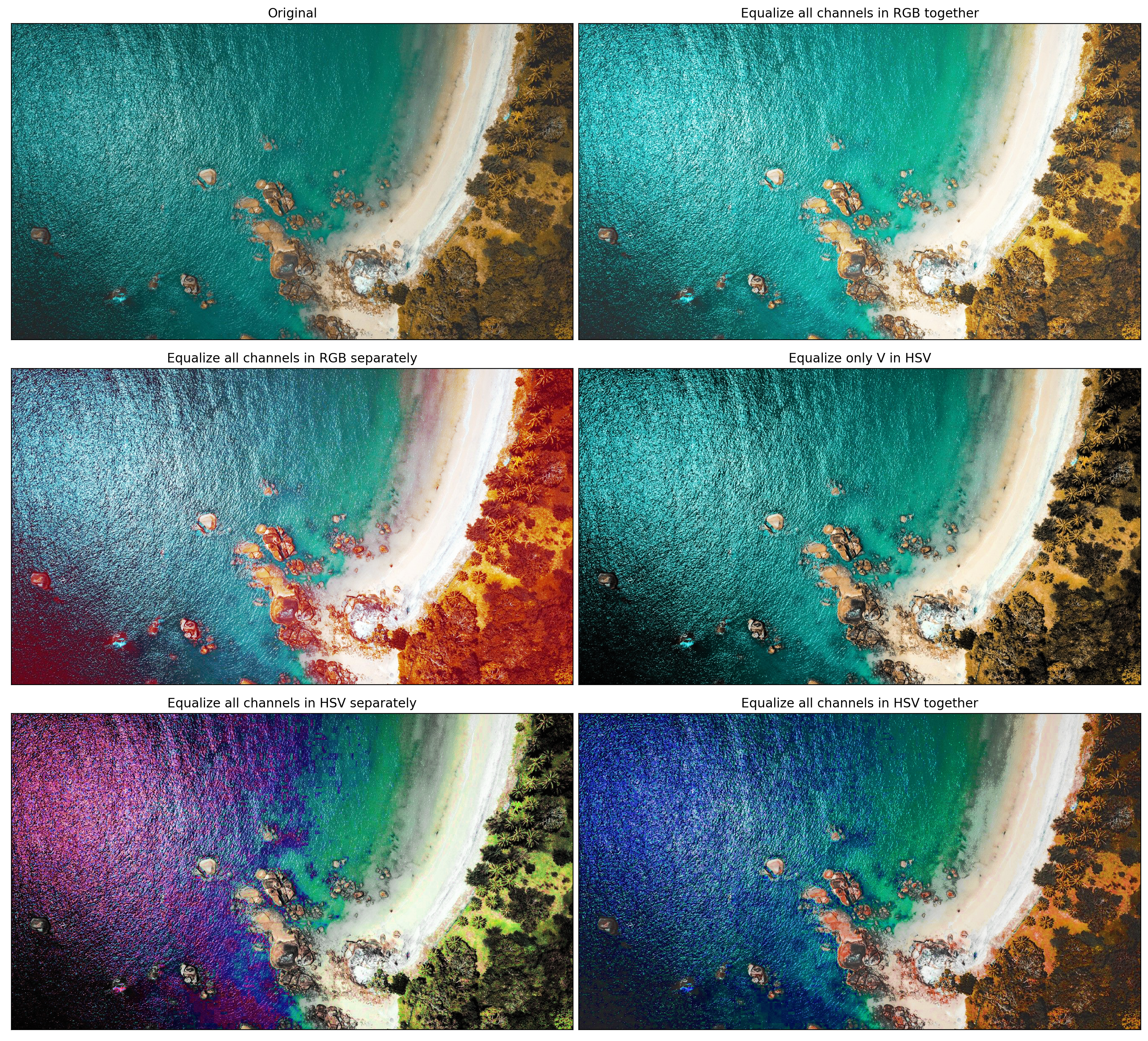
One small complication is that the above is defined only for gray-scaled images. If we intend to apply histogram equalization to multi-channel images, there are different possibilities to adapting the basic algorithm. Figure 2 shows some of them.
- We can apply equalization on each RGB channel separately, as if it's completely independent from the other channels. This would change the color balance and may result in completely unnatural colourings of the various objects in the image. For example, if the original image contains an overwhelming amount of pixels with close to 0 intensity in the red channel, then after equalization a lot of red would be inserted at the expense of the other over-abundant colours. This is the case with the image in Figure 2.
- We can apply equalization on all pixel intensities from all channels pooled together. In that case, we would be equalizing the distribution of all pixel intensities irrespective of the color channels. This tends to keep the color balance, but may produce images which are too bright, especially if some of the colour channels, like red, is altogether missing from the original image. This is what the library skimage is doing.
- We can convert the image to a different color space, where the colour channels are disentangled from the lightness channel, and apply the equalization over only the lightness channel. This is my personal preferred approach. Good candidate spaces are HSV (hue, saturatioon, value) and L*a*b*.

Now that we know how image equalization works and how it can be applied to multi-channel images, we can explore one particular improvement called CLAHE - contrast limited adaptive histogram equalization.
The standard algorithm described so far is global because it equalizes the intensity distribution across all pixels in the image. One limitation of this is that a small object which is bright in an image which is mostly dark will be enhanced less compared to the darker regions of the image. CLAHE fixes this problem by having local equalizations - for each pixel, compute the cdf in a square neighborhood around that pixel, and transform the central pixel's intensity as in the standard equalization, but using the cdf from the neighboring pixels only.
In practice, the neighborhoods tend to be fairly big. It's common to set them to be 1/8 of the image height by 1/8 of the image width. For those pixels whose neighborhoods extend beyond the image, the bordering columns and lines are mirrored, so as to not distort the distributions. If, instead, they were padded with zeros, this would introduce a sharp unwanted peak in the histograms.
Computing a separate equalization for every pixel provides maximal adaptation to local regions, but also requires maximal computation time. In practice, the algorithm is implemented using a lot of interpolation. This works as follows. The entire image is broken down into a number of (rectangular) blocks - for example 64 in total, 8 by 8 across the whole image. For each of these the cdf is computed and the intensity for the central pixel in each block is transformed. The new values for all other pixels are linearly interpolated.
Let's call the pixels in the center of each block central. For them we have computed the cdfs of their neighborhoods. Now consider a pixel with current intensity \(p\) and coordinates \((i, j)\). Assuming it is interior to the outermost block centers, we find the four closest central pixels \((i_{-}, j_{-}), (i_{-}, j_{+}), (i_{+}, j_{-}), (i_{+}, j_{+})\) and evaluate their cdfs at value \(p\). At this point we have an interior point \((i, j)\) and four surrounding points along with their four values. The value of point \((i, j)\) is then bilinearly interpolated from the surrounding points. Points \((i, j)\) which are beyond the outermost central pixels are linearly interpolated using only 2 central pixels. Finally, points near the corners are transformed using the cdf of the single nearest central pixel.

The adaptive modification in CLAHE also has a serious drawback. If the neighborhood region is fairly homogeneous, then a small range of values will be mapped to a large one. As a result, any noise in the input region will be amplified. This is where the contrast limited in CLAHE comes in.
The new pixel intensity is proportional to the cdf. Hence, if we want to limit the amount by which a pixel is modified it makes sense to limit the slope of the cdf. But the slope of the cdf at a given intensity \(p\) is proportional to the histogram value at \(p\). This motivates a clipping approach where we simply clip the histogram beyond a certain limit. For example, suppose for intensity \(p\) the probability from the histogram is \(0.04\). If we decide to clip the histogram at \(0.03\) then 1% of all pixels will not be used. What happens to that probability mass? It can be discarded or redistributed evenly to all other pixels in the neighborhood. All that matters is that we are clipping some of the peaks of the histogram which in turn produces, after renormalization, a cdf with a lower slope.
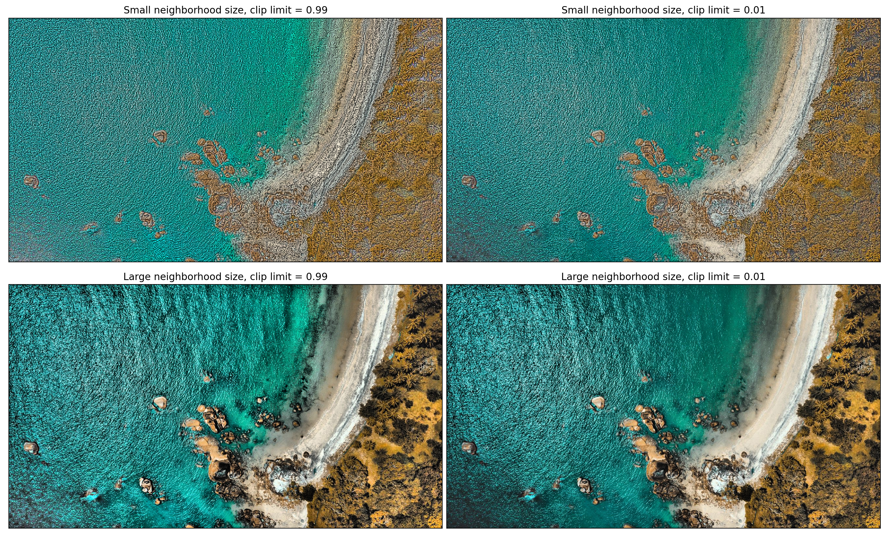
Figure 3 compares the outputs from various CLAHE settings. In the first row we use a very small neighborhood size of just \((5, 5)\). This produces an image which is very fine-grained - something typically undesirable. We test two clipping limits - \(0.99\) (essentially no clipping) and \(0.01\) (a lot of clipping). Note how the clipping prevents noise from being amplified, as specifically seen by the sandy beach. In the second row we compare much larger neighborhoods, which involves faster compute time due to less central pixels and more interpolation. Here we still see that a higher clipping limit produces more contrast but also more noise. While ultimately evaluation is subjective, the typically used neighborhood sizes are large and the clipping limits fairly small, as in the last image.