DINO, CLIP, PaliGemma
Here we take a look at some basic use-cases with DINOv2, Clip, and Google's new visual-language model PaliGemma 2. This is not meant to be a comprehensive overview of vision-language models. We will only dip our toes into this vast topic, which is only becoming more and more prominent in current AI. All these models can be considered foundational.
DINOv2 [1] is a very good model. It has found extremely wide applicability due to its strong generalization. It is a vision transformer, so nothing too exotic here, trained on a large-scale diverse dataset of very high quality. Of course the quality of the learned features greatly depends on the dataset. This is not a new insight. However, I was still very impressed by how much gain we can get from a well-constructed, curated, diverse dataset.
Let's look the large variant of DINOv2. It extracts \((14, 14)\) patches and projects them linearly, similar to the ViT [2]. In DINOv2 this happens simply using a big convolution layer whose kernel size and stride are both \((14, 14)\). This ensures that patches are non-overlapping and than no pixel remains unprocessed. Subsequently there are 24 encoder layers. In that sense the model is an encoder-only architecture. Each layer follows the transformer design - self-attention where all tokens attend to each other, layer norms for normalisation, residual connections, and a two-layer MLP with GELU activation.
The preprocessor usually needs to resize or crop the input images to be a mulitple of \(14\), so that it can be patchified evenly. A common resolution when using the large model is to resize images to \((448, 448)\). This results in \(448/14=32\) patches in each image axis, and a total of \(32*32=1024\) image patches, each representing a visual token. Additionally, a [CLS] token is added to represent any global information for the image that is not spatially localized. Hidden features throughout the model are of shape \((B, N+1, D)\) where \(D\) is the feature dimension and there are \(N+1\) total tokens.
We won't cover how the model is trained, which was explored previously. Instead, let's jump into the qualitative results. To visualize the learned features, we can do the following:
- We take the non-cls tokens of shape \((N, D)\) and do a single component PCA on them, producing \(N\) scalar numbers.
- The histogram of these numbers is usually multimodal and by rescaling and thresholding it, we can obtain those tokens which correspond to the background and the foreground of the image.
- We sulect only the tokens corresponding to the foreground and compute their 3-component PCA projection. We plot the foreground projections, of dimension 3, as a RGB image.
Various visualizations are shown in Figure 1. The projected features from step 3. are shown in the leftmost image, while the one next to it shows these features superimposed over the original image. Note that to get the shapes to be equal one needs to upsample and interpolate the token features, which are of shape \((\sqrt{N}, \sqrt{N})\), to the original image resolution. Note how different foreground objects within the same image are assigned relatively different features. Thus, within a single image the model "mostly" focuses on distinguishing the two main objects.
This is not the case if the model processes the objects independently. The model processes the last two images as independent samples in a batch and the elephant tokens from one image do not attend to the elephant tokens from the other image. Yet, when we do PCA, we compute the projection jointly for both samples, by flattening the batch dimension. This allows us to see that the model assigns the same semantic features to the same morphological parts of the animals. In other words, the model automatically learns part-of relationships and can perform dense point correspondences. For sparse correspondences, we can simply compute nearest neighbors.

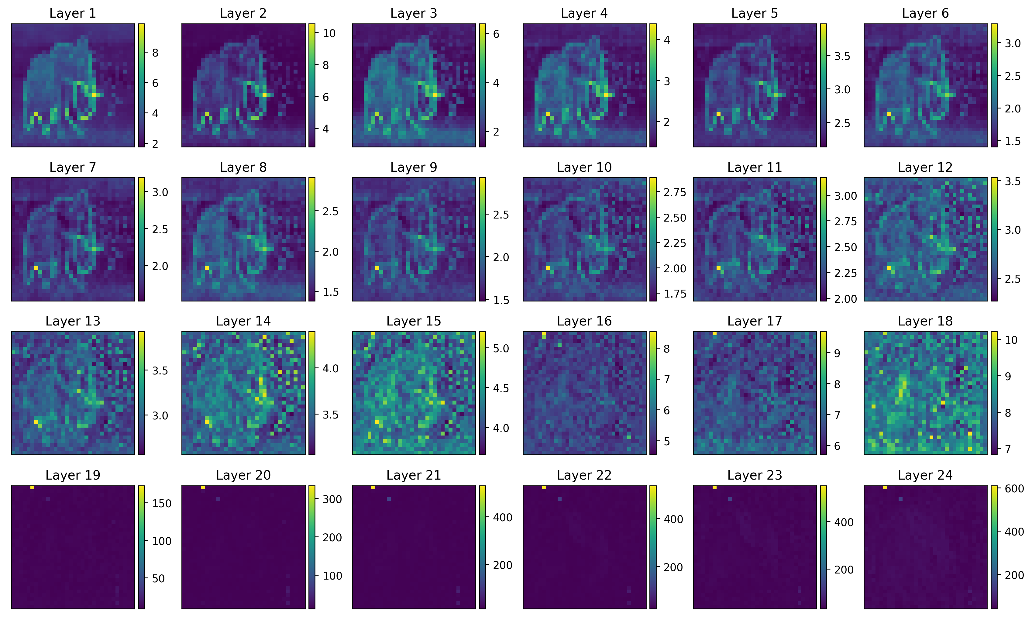
Now, something interesting happens if we look at the norm of the patch tokens throughout the layers, shown in Fig. 2. In the first layers, those tokens that correspond to patches with more edges or corners in them have a higher norm, which is reasonable. However, with the big models in the last few layers some tokens have a unproportionally large norm and may be considered artifacts.
These high norm tokens seem to occur in uniform color background areas and are otherwise random and few. In the Vision transformers need registers paper it is claimed that they result from the model repurposing them for other calculations [3]. Indeed, the hypothesis is that big models recognize that some tokens are redundant and too similar to their neighbors, and hence, they simply use them as storage containers for other features. The fix is simple - add a bunch of extra [reg] tokens that are learnable and fixed. This seems to remove the artifacts and improve performance on dense prediction tasks.

Note that the DINO features represent mostly part-of relationships. In certain tasks one might be interested in affordances, or articulations. Affordances are those actions that are "possible" on a given object, while articulations describe the degrees of freedom of an object's parts, such as rotation, translation, or deformation. Now, it is possible and useful to adapt the DINO features according to the desired task. E.g. imagine that a user requests those parts that would move in the same way under a certain action, or those object parts which effect some motion. In both cases the model should assign semantics depending on the task. This is a good paper where they do something similar [4]. By adopting another transformer that cross-attends over the image and text features, one can have those features corresponding to the handle of a knife light up when the affordance prompt is "hold", and to the blade of the knife when the affordance is "cut".
Now, another fundamental model is CLIP [5], the first big vision-language model and still one of the de facto standards. It consists of a text model and a vision model. The text model first uses a tokenizer to cut the text into tokens. Subsequently relevant dense vectors are retrieved based on the tokens and are fed into a encoder-only transformer. The vision model is a standard ViT. Finally, both the vision and text features are projected into the same dimension so that dot products can be computed as a form of similarity between text captions and images.
This design allows for open-vocabulary classification: you extract the image features corresponding to the [CLS] token from the vision backbone, and obtain the text features for a bunch of predefined text categories [dog, cat, cow, goat, ...], whatever they may be. To classify, simply assign that category that has the highest dot product with the image features. You can also do very very rough segmentation out of the box - simply don't use the [CLS] token, but use the individual patch tokens from the vision encoder. In general, this is the way to go, but results are very noisy and coarse-grained. It's better to add a mask-proposal network, like MaskCLIP does [6].
Finally, note that CLIP is a supervised model and as such plotting its features is mostly uninformative. It has been trained by matching images with their corresponding text captions. The features which we get at the last hidden layer are tuned precisely for this task and do not need to contain any meaningful spatial information, in the way that self-supervised methods like DINO do.
Let's also look at Google's new model PaliGemma 2 [7]. It's a proper VLM which uses the SigLIP-400m/14 vision encoder [8] and the Gemma 2 language model [9]. The architecture is quite straightforward:
- The SigLIP encoder is itself another transformer encoder but its main unique characteristic is the way it is trained. Usually, with CLIP training we use a softmax over all the image-text logits in the whole batch. With SigLIP the idea is to use a simple sigmoid, which has various benefits: it is more memory efficient and allows for a larger training batch size.
- The token features from the vision encoder are projected to the dimension of the language tokens. A single linear layer is sufficient here.
- The imput prompt is tokenized and the relevant dense embeddings are retrieved. They are then merged with the visual tokens. Specifically, the input prompt is processed to contain \(H/14 \times W/14\) special tokens in the beginning corresponding to the image. The dense vectors corresponding to them are replaced with the image token features to form an input of shape \((H/14 \times W/14 + T, D)\), where \(T\) is the length of the text part of the prompt. This big tensor is passed to the language model for autoregressive causal generation.
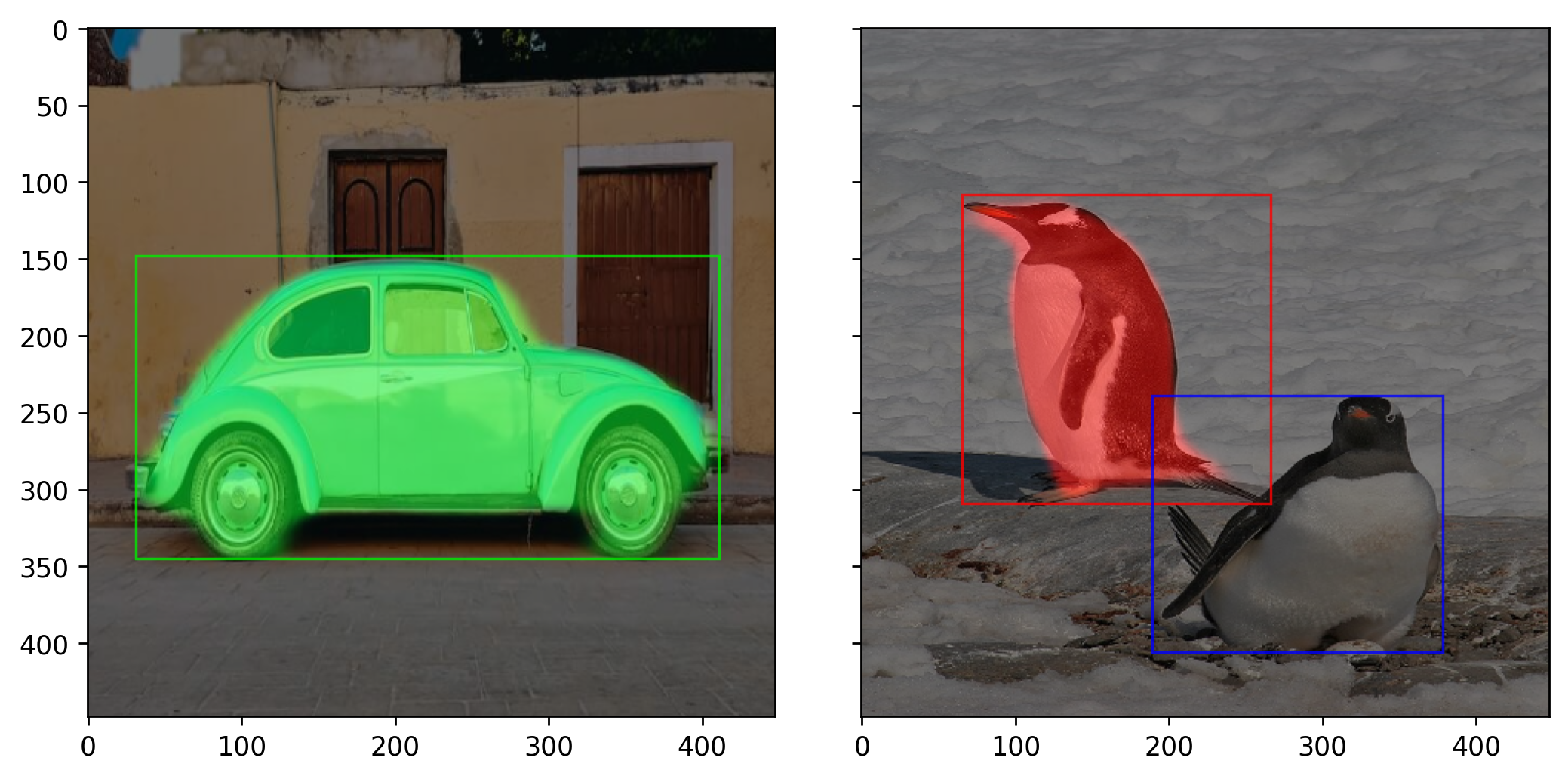
The token outputs of PaliGemma can be interpreted either as text or other modalities. In fact, being pretrained on multiple diverse tasks, the model can detect, segment, answer questions, and caption objects. It is quite impressive. The tokens generated by the LLM need to be parsed and represent codevectors that can be used by a VQ-VAE model to produce the segmentations [10]. Figure 3 shows a simple example. The inputs contain images and text prompts such as "segment the car" and "segment the penguin". The outputs are tokens decoded to strings like <loc0639>, <loc0540>, <seg0089>, <seg0102>. The location tokens are parsed to extract the bounding box coordinates. The segmentation tokens represent the codevector indices given to a decoder to output segmentation masks. 16 segmentation tokens are used to generate a mask of size \((64, 64)\), which is then resized and placed into the detection box for the visualization.

References
[1] Oquab, Maxime, et al. Dinov2: Learning robust visual features without supervision. arXiv preprint arXiv:2304.07193 (2023).
[2] Dosovitskiy, Alexey. An image is worth 16x16 words: Transformers for image recognition at scale. arXiv preprint arXiv:2010.11929 (2020).
[3] Darcet, Timothée, et al. Vision transformers need registers. arXiv preprint arXiv:2309.16588 (2023).
[4] Li, Gen, et al. One-shot open affordance learning with foundation models. Proceedings of the IEEE/CVF Conference on Computer Vision and Pattern Recognition. 2024.
[5] Radford, Alec, et al. Learning transferable visual models from natural language supervision. International conference on machine learning. PMLR, 2021.
[6] Zhou, Chong, Chen Change Loy, and Bo Dai. Extract free dense labels from clip. European Conference on Computer Vision. Cham: Springer Nature Switzerland, 2022.
[7] Steiner, Andreas, et al. PaliGemma 2: A Family of Versatile VLMs for Transfer. arXiv preprint arXiv:2412.03555 (2024).
[8] Zhai, Xiaohua, et al. Sigmoid loss for language image pre-training. Proceedings of the IEEE/CVF International Conference on Computer Vision. 2023.
[9] Team, Gemma, et al. Gemma 2: Improving open language models at a practical size. arXiv preprint arXiv:2408.00118 (2024).
[10] Ning, J., et al. All in Tokens: Unifying Output Space of Visual Tasks via Soft Token.. arXiv preprint arXiv:2301.02229.