Copulas and Tail Dependence
A portfolio can contain a hundred individually reasonable investments and still be one large bet. Mortgages issued in different cities might all depend on cheap refinancing. The individual risks look dispersed, but the circumstances that make them fail overlap. To understand diversification, we need to know both how bad each investment can get and how often they get bad together. We'll explore these concepts by looking at copulas, statistical objects that describe dependence between random variables.
What correlation leaves out. Imagine two assets whose returns have a correlation of 0.5. This tells us something useful about their linear co-movement. It does not tell us the probability that both lose more than 5% tomorrow. The correlation coefficient, being a single number, cannot fully represent all the information about how two assets depend jointly. Therefore, different joint distributions, with different tail shapes, can have the same correlation.
Within the Gaussian family, a joint distribution is completely specified by its means \(\boldsymbol{\mu}\) and covariance matrix \(\boldsymbol{\Sigma}\). Outside that family, means and covariances generally do not determine the distribution. Financial risk models often need precisely the information that they leave unspecified: simultaneous large losses, asymmetries between crashes and rallies, and clusters of defaults.
From returns to percentiles. Suppose \(X\) is one asset's return and \(F_X(x)=\Pr(X\leq x)\) is its cumulative distribution function. A return of \(-4\%\) means something different for a quiet bond fund than for a volatile stock. A percentile gives them a common scale. If \(F_X(-0.04)=0.01\), that return is at the first percentile: only 1% of the modeled outcomes are worse.
For continuous distributions, transforming a random return into its own percentile produces a uniform random variable. Do this for two assets:
Each percentile separately is uniform between zero and one. Their joint distribution \(C\) is the copula. Uniform does not mean independent: two assets can each visit every percentile equally often (the uniform part) while almost always visiting similar percentiles together (the dependent part).
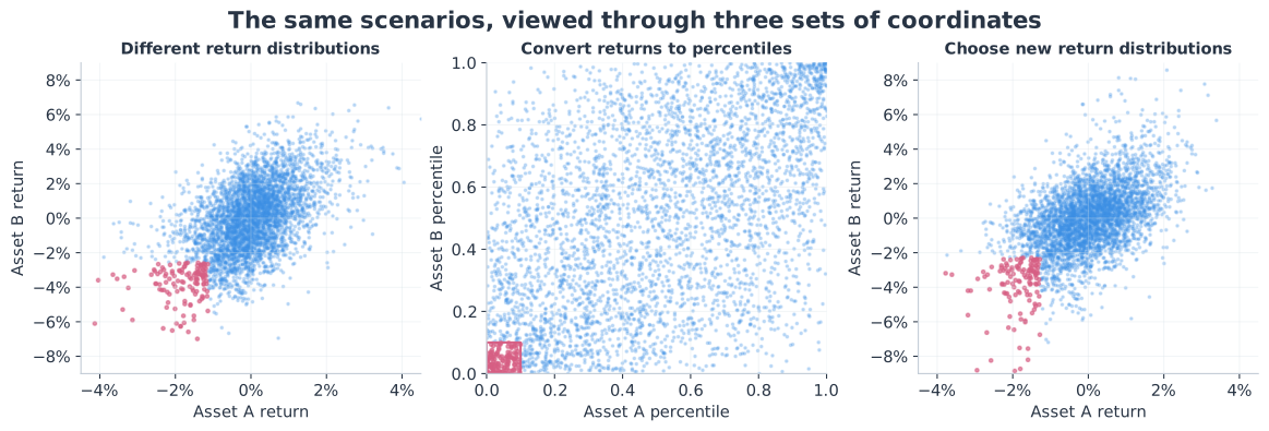
The lower-left corner of the unit square represents simultaneous bad outcomes. The upper-right represents simultaneous good ones. Let's see this visually. In Fig. 1 we simulate 4,000 paired returns: A has heavy-tailed returns with a standard deviation of 1%, and B has Gaussian returns with a standard deviation of 2%. We plot the returns on the left. The middle panel shows the outcomes in the percentile square \([0, 1]\times[0, 1]\). In the last panel we exchange the marginal distribution shapes while preserving each asset's standard deviation and the copula.
The glue between joint distributions and copulas is provided by Sklar's theorem, which says that a joint distribution can be written as
With continuous marginals, the copula is unique. The marginals \(F_X\) and \(F_Y\) describe each asset's individual behavior; the copula describes how their percentiles line up. In practice, this lets us specify the individual distributions and their dependence separately.
We can also run the construction backward. Draw dependent percentiles from a copula, then turn each percentile into a return using its asset's inverse CDF, or quantile function:
That is a complete recipe for generating joint scenarios. Choose how bad each asset can get, choose how their bad outcomes coincide, and simulate. The two choices interact in the resulting portfolio, but they are separate modeling inputs. Giving individual assets fat tails does not automatically give them joint tail dependence. Conversely, even assets with Gaussian marginals can have a copula that makes extreme losses cluster.
Measuring a shared crash. Let \(q=0.01\). Both assets being in their bottom 1% means \(U\leq q\) and \(V\leq q\). The copula immediately gives us the joint probability \(C(q,q)\). Divide by the probability that the first asset enters its tail to obtain
The first quantity answers a concrete question: given that one asset has a very bad outcome, how likely is the other to have one too? The limit \(\lambda_L\) is the lower tail dependence coefficient. Its upper-tail counterpart is \(\lambda_U=\lim_{q\downarrow0}\Pr(V>1-q\mid U>1-q)\). For a Gaussian copula with \(-1<\rho<1\), both limits are zero: the conditional probability of a companion extreme tends to zero as we move further into either tail.
If assets are independent, \(C(q,q)=q^2\) and the conditional probability is just \(q\). Knowing that one crashed gives no information about the other. If their percentiles are identical, \(C(q,q)=q\) and that conditional probability is one. A positive tail dependence coefficient describes something between these extremes: however far into the tail we go, a nonzero conditional chance of a companion extreme survives.
People sometimes call this “tail correlation,” but it is a conditional probability, rather than a Pearson correlation calculated on a subset of observations. The distinction matters. Also, the limit concerns equal percentiles, not equal percentage losses: the first percentile could mean a 3% loss for one asset and a 10% loss for another.
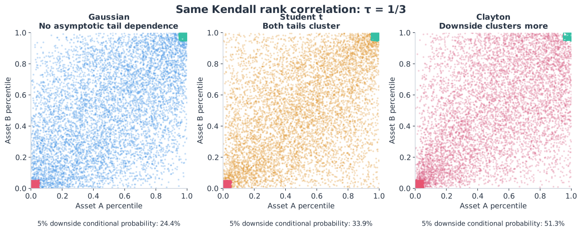
Different ways to move together. Fig. 2 illustrates how much structure can hide behind a summary measure of dependence. We show three copulas with the same Kendall rank correlation, \(\tau=1/3\). Kendall's tau is the probability that two independent scenarios order both assets in the same direction, minus the probability that they order them in opposite directions. Unlike ordinary Pearson correlation, it survives strictly increasing transformations of the marginals.
The Gaussian copula maps correlated standard normal variables \(Z_1,Z_2\) to percentiles:
where \(\Phi\) and \(\Phi_\rho\) are the standard and bivariate normal CDFs, the latter with correlation \(\rho\). Dependence is symmetric across tails, but for \(-1<\rho<1\), both tail coefficients are zero.
This does not make simultaneous large losses impossible or finite crash events independent. With \(\rho=0.5\), one asset entering its bottom 1% gives the other about a 13% chance of doing so, thirteen times the independent probability. Tail independence instead means that the conditional probability tends to zero as the percentile becomes more extreme.
The Student-t copula adds a shared random scale to the same normal pair. Draw an independent \(S\sim\chi^2_\nu\) and two correlated normals with correlation \(\rho\). Then set \(T_i=Z_i / \sqrt{S/\nu}\) and \(U_i=t_\nu(T_i)\). Here \(t_\nu\) is the univariate Student-t CDF. Small \(S\) amplifies both magnitudes, resembling a common volatility shock. For finite \(\nu\) and \(-1<\rho<1\), both tails have positive dependence. At \(\rho=0.5\) and \(\nu=4\), the conditional probability is about 29% at the bottom-1% threshold and tends to 25%. Even \(\rho=0\) leaves tail dependence in the finite-degree t model: zero directional correlation does not remove the shared scale.
The Clayton copula, with \(\theta>0\), is
Dependence concentrates in the lower tail: \(\lambda_L=2^{-1/\theta}\) and \(\lambda_U=0\). This suits crashes that cluster more than rallies. Other copulas, like Gumbel, instead concentrate dependence in the upper tail.
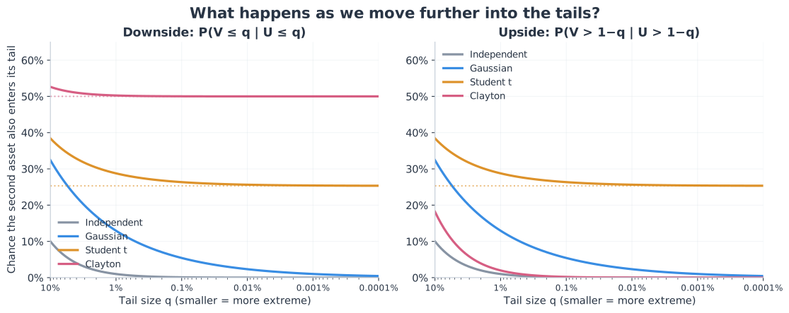
Fig. 3 captures the distinction visually. The models have the same rank correlation, but their answers to “how likely is a companion crash?” diverge as the threshold becomes more severe. At the bottom-1% threshold, the joint probabilities are approximately 0.13% for Gaussian, 0.29% for t, and 0.50% for Clayton. Independence gives 0.01%.
What happens to a portfolio? Consider a portfolio split equally between two assets. Give both exactly the same heavy-tailed marginal return distribution: Student-t with five degrees of freedom, zero mean, and a 1% standard deviation. Change only their copula. The one-period portfolio loss, expressed as a fraction of its initial value, is
Value-at-Risk \(\operatorname{VaR}\) is a loss threshold: 99% VaR is exceeded in 1% of the modeled scenarios. Expected shortfall \(\operatorname{ES}\) asks how large the loss is on average within that worst 1%. The conditional-expectation formula above applies to our continuous loss distribution.
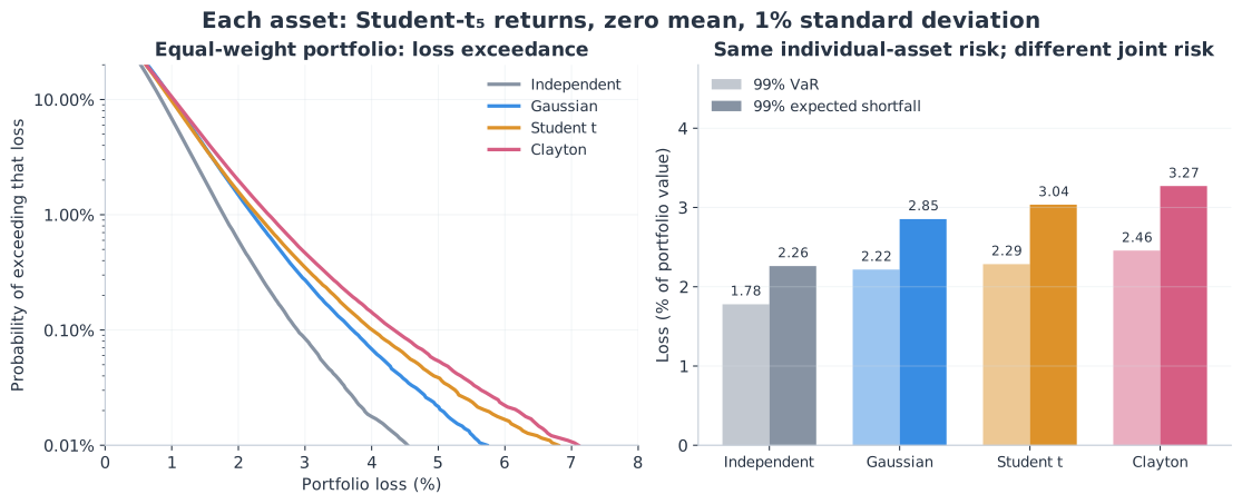
The individual investments have not become more volatile in the t and Clayton experiments. Their worst outcomes simply coincide more often. Hence, diversification loses some of its protection, because the second asset is less likely to offset the first asset's loss. The estimated 99% expected shortfall rises from 2.85% under Gaussian dependence to 3.04% under t dependence and 3.27% under Clayton dependence.
There is no general rule that one family always produces the largest portfolio VaR. Weights, thresholds, marginal distributions, and the rest of the joint distribution all matter. Even knowing the tail dependence coefficient does not determine a portfolio's risk. The useful practice is to compare the loss distributions generated by plausible dependence assumptions, rather than convert one coefficient into a universal risk multiplier.
Example application in credit. Let's now consider loans and pools of loans. A loan's default probability is a marginal quantity. A pool's loss distribution also depends on which loans default together. For \(N=100\) equally sized loans with a 2% default probability over a chosen horizon, represent default by \(U_i\leq0.02\). The expected number of defaults is always two:
That equality does not require independence. It follows from adding expectations. Dependence changes the distribution around the average, potentially producing many quiet scenarios and occasional clusters of defaults.
For the next experiment, each loan has one Gaussian latent score \(Z_i=\sqrt{\rho}M+\sqrt{1-\rho}\epsilon_i\). The shared \(M\) represents common economic conditions; each \(\epsilon_i\) represents borrower-specific circumstances. These inputs are independent standard normals. "One factor" means one shared influence across all 100 loan scores, with \(\rho\) controlling their correlation. Now set \(U_i=\Phi(Z_i)\), where \(\Phi\) is the standard normal CDF. Loan \(i\) defaults when \(U_i\leq0.02\), giving it a 2% default probability. Each scenario counts defaults across the 100 loans. A very negative \(M\) lowers all scores, making clustered defaults more likely. The t version divides all scores by one additional common random scale before converting them to percentiles using the Student-t CDF. Both use \(\rho=0.5\); their continuous latent percentiles have pairwise Kendall's tau of \(1/3\).
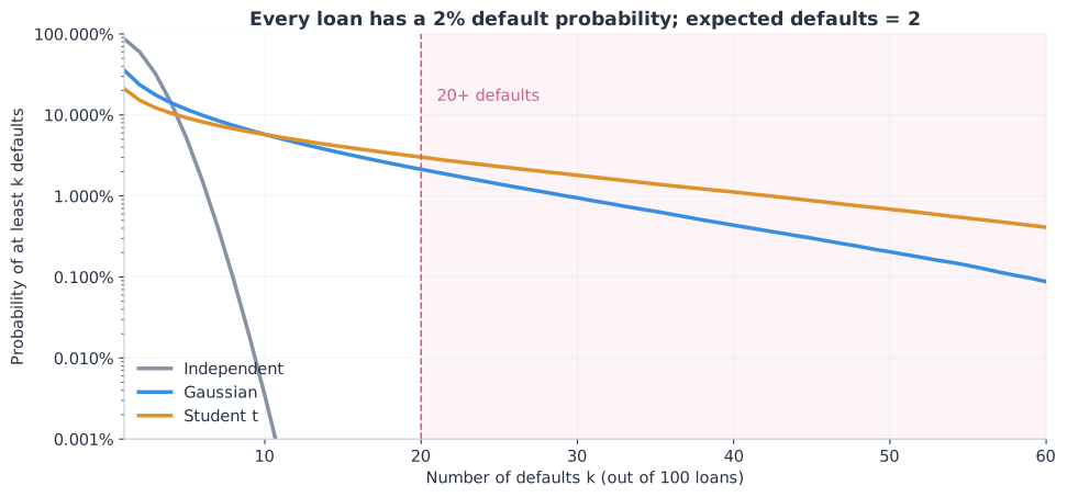
A tranche specifies who absorbs which part of a pool's losses. An equity tranche takes losses first; a senior tranche begins losing principal only after lower layers are exhausted. Assuming equal exposures and no recovery, a layer that starts absorbing losses at 20% of pool principal is reached at 20 defaults and begins taking losses at the twenty-first. Its exposure depends on the far right of this figure, even though the expected total pool loss is unchanged.
In this experiment, the probability of at least 20 defaults is about 2.13% under Gaussian dependence and 3.01% under t dependence. With independent defaults it is roughly \(1.2\times10^{-14}\). Dependence can therefore change what looks like an almost impossible pool outcome into a material risk, without changing a single loan's default probability.
Copulas in practice. We start with aligned observations, such as daily returns for the assets. We fit a marginal distribution to each asset's returns and convert the observations to percentiles. Next, we choose candidate copula families and estimate their parameters, usually by maximizing the likelihood of the observed percentile pairs. A Gaussian fit estimates the latent correlation; a t fit also estimates degrees of freedom. We compare the fitted models on later data, including how well they predict joint extremes.
The fitted dependence can be used for risk management: draw joint percentiles, convert them back into returns, and calculate portfolio losses. This helps assess whether adding a position improves diversification and how much exposure the portfolio can support.
This assumes the estimated marginal distributions and dependence remain relevant over the decision horizon. A shorter rolling estimation window emphasizes recent conditions but leaves fewer observations for fitting. The copula family also imposes structure: Gaussian dependence excludes asymptotic tail dependence, while the t construction above gives all assets a shared random scale. Unfortunately, crash observations are usually scarce, which leaves these assumptions weakly tested, even when the overall fit looks good. The next crash may reveal how many of your different investments were the same bet all along.