Can LLMs Learn to Reason End-to-End?

I was recently thinking about reasoning models and why RL methods like GRPO have become so prominent in that context. Previously, people were finetuning LLMs on step-by-step reasoning traces, yet this can hardly be called "learning to reason", as it's rather about learning to reproduce the reasoning patterns of some other expert. With RL for LLMs the paradigm has shifted and now the model can, in principle, discover the right reasoning patterns for the task. Yet, there are still lots of nuances. Here we consider a simple question: can LLMs learn the best reasoning patterns in an end-to-end manner? By understanding this we'll see precisely how different model designs and training paradigms fit together, like pieces of a puzzle.

Pretraining

We'll explore the advantages and disadvantages of current LLMs in a bottom-up manner. Imagine you want to train a new LLM. To endow it with general knowledge of facts and concepts, and the ability to construct cohesive linguistic phrases, you need to first pretrain it. This involves collecting a huge internet-scale training corpus of exemplary text data, and teaching the model to reproduce the text distribution induced from it. The training process does not involve sampling.

Concretely, if we are given a text document, we tokenize it and obtain, say, $T$ tokens representing the document. They are given to the language model, which retrieves their dense embeddings, and pushes them through the transformer layers. At the end we end up with some logits of shape $(T, V)$ where $V$ is the vocabulary size. We apply a softmax over $V$, obtaining $T$ categorical distributions. The targets will be the tokens of the document shifted forward by one. Now, we want the model to learn the true distribution of the next tokens. Thus, we can minimize the KL divergence $D_{KL}(P \ || \ Q_\theta)$ where $P$ is the ground-truth distribution of the next-token and $Q_\theta$ is the predicted one (from the softmax). The KL between two categorical distributions $P$ and $Q$, where the $P$ distribution is one-hot (at index $j$), is a cross-entropy term:

$$ D_{KL}(P \ || \ Q_\phi) = \sum_{i=1}^V p_i \log\left(\frac{p_i}{q_i}\right) = 1\cdot \log\left(\frac{1}{q_j}\right) + \sum_{i \ne j} 0 = -\log(q_j). $$

The pretraining optimization chooses those LLM weights $\theta$ that maximize the log-likelihood of seeing the right tokens, which are the same as those minimizing the negative log-likelihood. We can augment the token sequence with BOS and EOS tokens to easily handle the beginning and end. If $q_{t, j}$ represents the predicted probability that the $t$-th next-token is the $j$-th one from the vocabulary, where $j$ is the correct one, the problem to solve can be written simply as:

$$ \min_\theta \ \mathcal{L}_\text{pretrain} = -\frac{1}{T} \sum_{t = 1}^T \log(q_{t, j}). $$

Note the main characteristic of pretraining: it does not involve any generation. The LLM only ever gets to see the true sequences, and starting from them, learns to predict the next tokens.

Fine-Tuning

Okay, now that the LLM has some general language speaking capabilities, we'd like to adapt it for certain convenient behavioral patterns, such as responding to questions and following instructions. This would be the instruction-tuning phase. We collect curated sequences representing good conversations between the user and the model and simply train it to reproduce them, as above. Different from the pretraining corpus, in these training documents we have explicit queries directed to the model itself, along with explicit exemplary answers. Prompt templates start to appear so that the LLM can get used to the conversation format. By training on such carefully-curated datasets, the model can pick up convenient patterns in how to structure its answers, how to present them, when to refuse answering, and so on.

This type of finetuning has been the go-to method for adapting LLMs to novel specific tasks. To help the model think step-by-step, finetune it on a dataset of step-by-step solutions. To make it avoid certain questions, train it on a toxic dataset of dangerous queries and limited answers such as "I cannot help you with that". To help it use tools, train it on a dataset of answers where the tool calls are explicitly annotated. Domain adaptation, persona tuning, style... the list goes on.

Preference Optimization

But what happens when you don't have ground-truth data for the particular characteristic of the answer we're looking for? In that case you cannot supervise its reconstruction. That's where techniques like DPO [1] come in. They represent a different training paradigm, often called preference optimization.

Imagine you want to train the model to respond in a way that maximizes "user engagement". However, for a particular prompt $x$ you don't know which answer will maximize engagement. You can only ask people to compare different answers and assess them in relation to each other. So generally, while we don't have ground-truth data, we assume it's possible to recognize a good solution from a bad one. That is, when presented with two answers, it's possible to rank them and change the LLM weights $\theta$ so as to increase the probability of reconstructing the good one. Consider a dataset where each sample contains a prompt $x$, a preferred answer $y^+$ and a less-preferred one $y^-$. DPO [1] is a technique that increases the likelihood of the preferred answers:

$$ \min_\theta \ \mathcal{L}_\text{DPO} = -\log \sigma \left(\beta \left[\log\frac{\pi_\theta(y^+|x)}{\pi_\text{ref}(y^+|x)} - \log\frac{\pi_\theta(y^-|x)}{\pi_\text{ref}(y^-|x)}\right] \right). $$

This loss boosts the probability $\pi_\theta(y^+|x)$ of the preferred response compared to that of the rejected one, all relative to some reference policy $\pi_\text{ref}(\cdot)$ which is usually a copy of the model weights after finetuning and before this preference optimization process has started. This reference policy pops up in the objective because usually we don't want the learned policy $\pi_\theta$ to deviate too far from the initial language model (there is a KL term in the derivation). If it does, the model may start losing its linguistic cohesiveness. The sigmoid $\sigma(\cdot)$ simply maps score differences into probabilities, so that the whole loss becomes a negative log-likelihood.

In DPO there is still no reinforcement learning - no trial and error, and no token generation to sample answers. Given the responses $y^+$ and $y^-$ we can compute their log-probs by directly summing the log-probs of their tokens. Thus, DPO enables preference optimization (with the underlying framework called Bradley-Terry) in a supervised manner.

Reinforcement Learning

For a more ambitious setting, we'd want to teach the model how to "reason". With LLM it has become the norm to call reasoning the process of outputting multiple tokens, used effectively as scratch tokens, before providing a final answer. Those "thinking tokens" can represent any kind of meandering chain of thought in which you try out one approach, backtrack, reasses, replan, try another approach, and so on. The models are usually prompted to output this kind of reasoning within <think>...</think> tags, followed by the final answer.

In DeepSeek-R1 [2] it was beautifully shown how training with RL can allow the model to develop useful reasoning patterns for logical and mathematical tasks. There (in DeepSeek-R1-Zero) we don't have a dataset of good reasoning prompts. What's available is only a way to evaluate whether the final answer is correct or not. Hence you cannot reconstruct any reasoning chains and you need to sample multiple outcomes, assess them using the reward engine, and increase/decrease the likelihood of the good/bad ones - a totally different paradigm than DPO.

This difference is crucial. If you supervise the model on reasoning traces, you're directly teaching it what to think. It that sense, supervised learning kills its creativity. With RL however, you are allowing the model to discover what to think, which is a much harder optimization, but it allows the model to come up with new ways of thinking beyond those in a collected dataset.

GRPO [3], the algorithm at hand, works as follows. First, for the prompt $x$ we sample $G$ response outcomes from the LLM, $o_1, ..., o_G$. Each could contain different reasoning patterns before the final answer. These responses are called a group. We use the reward engine to check if the final answer is correct, obtaining rewards $r_1, ..., r_G$. Further, we compute advantages $A_1, ..., A_G$ by normalizing the rewards across the group. This is a big difference compared to the well-known PPO [4]. In PPO rewards are per-step and we compute the advantages using $\text{GAE}(\lambda)$, normalized across the batch. In GRPO rewards are per-entire-sequence and are normalized within each group. Moreover, in PPO there is a learned critic, while here there isn't. Relativity results from sampling many outcomes for the same query $x$ and judging them relatively to each other.

Once we compute the advantages, we increase the likelihood of the generated sequences according to their advantage. An $o_i$ that performs better than the other ones will have its likelihood boosted, while one that performs worse, suppose $o_j$, will have its likelihood reduced. Whatever reasoning patterns are in $o_i$ will get reinforced. The optimization bundles this logic within a PPO-style update:

$$ \begin{align} \max_\theta \ \mathcal{L}_\text{GRPO} &= \frac{1}{G}\sum_{i=1}^G \bigg( \min \Big(\rho(o_i)A_i, \text{clip}\big(\rho(o_i), 1 - \epsilon, 1 + \epsilon\big) A_i \Big) - \beta D_{KL}(\pi_\theta \ || \ \pi_\text{ref}) \bigg) \\ \text{ with } \rho(o_i) &= \frac{\pi_\theta(o_i | x)}{\pi_{\theta_\text{old}}(o_i | x)} \text{ and } A_i = \frac{r_i - \text{mean}(r_1, ..., r_G)}{\text{std}(r_1, ..., r_G)}.\\ \end{align} $$

The beauty of this approach is that those thinking tokens that display any reasoning patterns that are useful, such as checking your solution, backtracking, finding similarities to other problems, will be reinforced. The model is free to experiment using trial-and-error generation, until it finds those reasoning traces that work. In practice some additional tricks are used to facilitate the search. One example is supervising the reasoning traces, which kind of defeats the purpose...

Note that in DeepSeek-R1 the rewards are rule-based - they encourage the model to provide the right answer and to correctly format its outputs. For math and coding, rewards are discrete, often binary, and come from checking whether the final answer is correct, whether any unit tests succeed, or whether the output can be parsed without errors. Hence, why do we use RL for this? Because the rewards are non-differentiable by design and we cannot compute $\partial r_i / \partial \theta$.

Differentiable Simulation

But what if the rewards are differentiable? We know that for example with differentiable simulation you can train policies without the sample-inefficient trial-and-error complexity of RL. The big difference is that non-differentiable rewards provide only evaluative feedback, telling you whether something is good or bad, whereas differentiable rewards provide instructive feedback. That is, the gradient tells you exactly how you should change your controls so that this reward increases as fast as possible. So, can we avoid GRPO when training reasoning LLMs if the rewards are differentiable? With this question we're entering uncharted waters.

I was recently trying to figure out a setup where a VLM is tuned to reason for end-to-end driving in a simulator. Specifically, the VLM takes in six-or-so images $x_t$, representing the scene around the ego-vehicle, produces some reasoning tokens <think>...</think>, and based on them finally outputs an action $a_t$. The action goes into the simulator $\text{Sim}$ which returns the next state $y_{t+1}$, over which a loss is calculated. The question is: how do we learn the right thinking patterns so that conditioned on them, the produced action $a_t$ results in the best outcome $y_{t+1}$?

In that setting the simulator is differentiable and we can get $\partial y_{t+1} / \partial a_t$, but we still cannot obtain $\partial a_t / \partial \theta$ because the LLM samples discrete tokens autoregressively and for any kind of derivative we need to have continuous outputs. So in the end, even if the rewards are differentiable or we have some differentiable loss over the sampled outputs, we still need to use RL methods like GRPO to train the LLM. The real fault here is in how LLMs use discrete tokens during the generation. If this were not the case, we'd be able to learn in an end-to-end manner the optimal <think>...</think> tokens that, when conditioned on, produce the right actions.

Fig. 1. What does end-to-end learnable reasoning look like? In the case of an action reasoner within an environment, the loss is formulated as the difference between a realized state and a desired one. For end-to-end learnable reasoning, gradients from that loss need to flow through the dynamics, the actions, and the thinking tokens, reaching the model's parameters $\theta$. What prevents this in practice is the variable-length sequence generation and the discrete nature of the tokens.

This is the core of end-to-end reasoning. If tokens are generated in a differentiable way, we'd be able to backpropagate any downstream gradients through them, which will enable easily finding the optimal thinking tokens for that task, without the need for trial-and-error RL. The benefits:

End-to-end trainable: single unified computation graph, gradients flow all the way back;
No trial-and-error search: downstream loss provides instructive feedback on how to improve;
Discoverable reasoning patterns: thinking tokens not supervised, but tuned for specific task;

LLMs With Differentiable Rollout?

For the most efficient training we need both the rewards and the token rollout to be differentiable. Let's see how we can make the rollout differentiable.

Suppose the logits are $\ell_1, ..., \ell_V \in \mathbb{R}^V$ and dense embeddings for tokens are denoted as $z \in \mathbb{R}^D$. A first idea is to do $z = \text{softmax}(\ell_1, ..., \ell_V)^T \mathbf{E}$, where $\mathbf{E} \in \mathbb{R}^{(V, D)}$ is the embedding matrix for all tokens. This is fully-differentiable and deterministic but the output is the expected embedding under the categorical. This is not what language modeling is about, as we need to be able to sample from the categorical. Also, at inference if we switch to hard sampling, we'll introduce train-test mismatch, which can hurt performance.

To model actual sampling, we need to reparametrize the categorical, which is done using the Gumbel-softmax trick. We start with the logits over the vocabulary $\ell \in \mathbb{R}^V$. Sample a vector of uniform noise $u_i \sim \text{Uniform}(0, 1)$ and compute $g_i = -\log(-\log u_i), \forall i$, which gives us Gumbel noise. We add the Gumbel samples to the logits and scale by a temperature $\tau$, obtaining $\tilde{\ell}_i = (\ell_i + g_i)/\tau$. Now, it's known that the argmax of this is distributed as a categorical,

$$ \text{argmax}_i \ \ \tilde{\ell}_i = (\ell_i + g_i) \sim \text{Categorical}\big(\text{softmax}(\ell_1, ..., \ell_V)\big). $$

Then, we need to formulate a soft sample from the categorical, for which we take $\text{softmax}(\tilde{\ell}_1, ..., \tilde{\ell}_V)$. The final output is $z = \text{softmax}(\tilde{\ell}_1, ..., \tilde{\ell}_V)^T \mathbf{E}$, where $\tilde{\ell}_i = (\ell_i + g_i)/\tau$ and $g_i \sim \text{Gumbel}(0, 1)$. This represents a soft sample from the categorical embeddings, according to the logits $\ell$. If the temperature $\tau$ is large, $z$ is essentially a mixture of embeddings and any gradients will be biased. If $\tau$ is very small, close to $0$, $z$ does correspond to one particular embedding, but the variance in the gradients can explode. Hence, there's no easy way out. The Gumbel-softmax trick is a useful way to obtain the derivative $\partial z / \partial l_i$, but its bias and variance will make training either meaningless or difficult. If this approach worked at scale, we would have seen it already applied to the big LLMs.

Language Diffusion

Another interesting direction is language diffusion models. The appeal is that diffusion may offer a route to differentiable token rollout. A first idea is to run diffusion not over discrete token IDs but over their continuous embeddings. This is the approach in DiffuSeq [5]. Noise is added directly to high-dimensional embeddings, and the model learns to denoise them. At test time, the final denoised embedding is mapped to the nearest discrete token by rounding. The drawback is limited flexibility: generation is always padded up to a fixed maximum length, and variable-length answers are handled only by mapping some denoised embedding to the EOS token, which can occur earlier or later in the sequence but never beyond the fixed cap.

In the large-model era, LLaDA [6] adopts a mechanism that resembles masked language modeling (MLM). We start from an input sequence $x_0$ and sample a time $t \sim \text{Uniform}(0,1)$. Each token is masked independently with probability $t$, producing a corrupted sequence $x_t$. A predictor $p_\theta(\cdot|x_t)$ then fills in the missing tokens. The architecture is a standard transformer with a softmax output, but unlike autoregressive LLMs it does not use causal masking - each position attends bidirectionally across the whole sequence. The mask token MASK has its own learned embedding. At inference, we begin with all tokens masked and iteratively denoise: at each step, a fraction of predicted tokens are remasked for further refinement.

Compared to autoregressive LLMs, LLaDA cannot benefit from KV caching, which is a important engineering problem. With autoregressive LLMs, due to the causal generation, the KVs of past tokens don't change and can be stored and reused. With LLaDA however, since the token at position $i$ can change from one denoising step to another, you need to recompute all keys and values, so it makes no sense to store them in a cache.

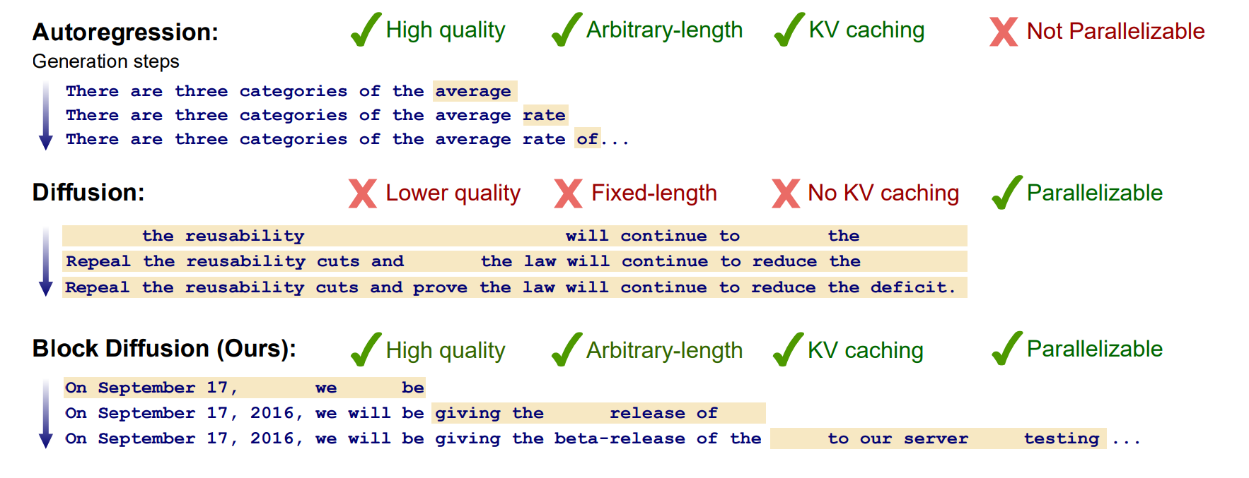
What is much more exciting is called block diffusion [7]. It's a mixture between autoregressive modeling of blocks of tokens, and diffusion generation within each block. It has its selling points: first, you can do KV caching, as the tokens outside the current block don't change. Second, you can do arbitrary-length generation due to the autoregressive part. Third, you can parallelize the generation of those tokens within the current block, due to the diffusion design. Unfortunately, it still samples from the discrete tokens through which you can't differentiate.

From the big tech labs, Gemini Diffusion looks promising although its detailed architecture and design are still unclear. The main questions are whether diffusion as a generative paradigm can be scaled to huge models, and whether performance-enhancing chain-of-thought and test-time compute strategies can be employed. Exciting times ahead.

Conclusion

Dataset limitations and architectural design decisions influence current LLM training approaches. The ideal case of end-to-end learnable reasoning, that is not trained to reproduce chains-of-thought but discover them, is still not achievable. With supervised finetuning you do not discover the optimal reasoning patterns. With RL you do, but it's hard and sample-inefficient due to the trial-and-error involved. What prevents fully end-to-end training is, first, the variable length generation and second, the discrete nature of tokens. Even with tokens relaxed into continuous hidden states, the decision of when to stop generating is itself discrete and you can't backprop through it. Diffusion might be an option but it will require architectural changes.

References

[1] Rafailov, Rafael, et al. Direct preference optimization: Your language model is secretly a reward model. Advances in neural information processing systems 36 (2023): 53728-53741.
[2] Guo, Daya, et al. Deepseek-r1: Incentivizing reasoning capability in llms via reinforcement learning. arXiv preprint arXiv:2501.12948 (2025).
[3] Shao, Zhihong, et al. Deepseekmath: Pushing the limits of mathematical reasoning in open language models. arXiv preprint arXiv:2402.03300 (2024).
[4] Schulman, John, et al. Proximal policy optimization algorithms. arXiv preprint arXiv:1707.06347 (2017).
[5] Gong, Shansan, et al. Diffuseq: Sequence to sequence text generation with diffusion models. arXiv preprint arXiv:2210.08933 (2022).
[6] Nie, Shen, et al. Large language diffusion models. arXiv preprint arXiv:2502.09992 (2025).
[7] Arriola, Marianne, et al. Block diffusion: Interpolating between autoregressive and diffusion language models. arXiv preprint arXiv:2503.09573 (2025).